hypothesis testing with one sample

Want to create or adapt books like this? Learn more about how Pressbooks supports open publishing practices.

11 Hypothesis Testing with One Sample

Student learning outcomes.

By the end of this chapter, the student should be able to:

• Be able to identify and develop the null and alternative hypothesis
• Identify the consequences of Type I and Type II error.
• Be able to perform an one-tailed and two-tailed hypothesis test using the critical value method
• Be able to perform a hypothesis test using the p-value method
• Be able to write conclusions based on hypothesis tests.

Introduction

Now we are down to the bread and butter work of the statistician: developing and testing hypotheses. It is important to   put this material in a broader context so that the method by which a hypothesis is formed is understood completely. Using textbook examples often clouds the real source of statistical hypotheses.

Statistical testing is part of a much larger process known as the scientific method. This method was developed more than two centuries ago as the accepted way that new knowledge could be created. Until then, and unfortunately even today, among some, “knowledge” could be created simply by some authority saying something was so, ipso dicta . Superstition and conspiracy theories were (are?) accepted uncritically.

The scientific method, briefly, states that only by following a careful and specific process can some assertion be included in the accepted body of knowledge. This process begins with a set of assumptions upon which a theory, sometimes called a model, is built. This theory, if it has any validity, will lead to predictions; what we call hypotheses.

As an example, in Microeconomics the theory of consumer choice begins with certain assumption concerning human behavior. From these assumptions a theory of how consumers make choices using indifference curves and the budget line. This theory gave rise to a very important prediction, namely, that there was an inverse relationship between price and quantity demanded. This relationship was known as the demand curve. The negative slope of the demand curve is really just a prediction, or a hypothesis, that can be tested with statistical tools.

Unless hundreds and hundreds of statistical tests of this hypothesis had not confirmed this relationship, the so-called Law of Demand would have been discarded years ago. This is the role of statistics, to test the hypotheses of various theories to determine if they should be admitted into the accepted body of knowledge; how we understand our world. Once admitted, however, they may be later discarded if new theories come along that make better predictions.

Not long ago two scientists claimed that they could get more energy out of a process than was put in. This caused a tremendous stir for obvious reasons. They were on the cover of Time and were offered extravagant sums to bring their research work to private industry and any number of universities. It was not long until their work was subjected to the rigorous tests of the scientific method and found to be a failure. No other lab could replicate their findings. Consequently they have sunk into obscurity and their theory discarded. It may surface again when someone can pass the tests of the hypotheses required by the scientific method, but until then it is just a curiosity. Many pure frauds have been attempted over time, but most have been found out by applying the process of the scientific method.

This discussion is meant to show just where in this process statistics falls. Statistics and statisticians are not necessarily in the business of developing theories, but in the business of testing others’ theories. Hypotheses come from these theories based upon an explicit set of assumptions and sound logic. The hypothesis comes first, before any data are gathered. Data do not create hypotheses; they are used to test them. If we bear this in mind as we study this section the process of forming and testing hypotheses will make more sense.

One job of a statistician is to make statistical inferences about populations based on samples taken from the population. Confidence intervals are one way to estimate a population parameter. Another way to make a statistical inference is to make a decision about the value of a specific parameter. For instance, a car dealer advertises that its new small truck gets 35 miles per gallon, on average. A tutoring service claims that its method of tutoring helps 90% of its students get an A or a B. A company says that women managers in their company earn an average of $60,000 per year.

A statistician will make a decision about these claims. This process is called ” hypothesis testing .” A hypothesis test involves collecting data from a sample and evaluating the data. Then, the statistician makes a decision as to whether or not there is sufficient evidence, based upon analyses of the data, to reject the null hypothesis.

In this chapter, you will conduct hypothesis tests on single means and single proportions. You will also learn about the errors associated with these tests.

Null and Alternative Hypotheses

The actual test begins by considering two hypotheses . They are called the null hypothesis and the alternative hypothesis . These hypotheses contain opposing viewpoints.

Since the null and alternative hypotheses are contradictory, you must examine evidence to decide if you have enough evidence to reject the null hypothesis or not. The evidence is in the form of sample data.

Table 1 presents the various hypotheses in the relevant pairs. For example, if the null hypothesis is equal to some value, the alternative has to be not equal to that value.

NOTE                                                                             

We want to test whether the mean GPA of students in American colleges is different from 2.0 (out of 4.0). The null and alternative hypotheses are:

We want to test if college students take less than five years to graduate from college, on the average. The null and alternative hypotheses are:

Outcomes and the Type I and Type II Errors

The four possible outcomes in the table are:

Each of the errors occurs with a particular probability. The Greek letters α and β represent the probabilities.

By way of example, the American judicial system begins with the concept that a defendant is “presumed innocent”. This is the status quo and is the null hypothesis. The judge will tell the jury that they can not find the defendant guilty unless the evidence indicates guilt beyond a “reasonable doubt” which is usually defined in criminal cases as 95% certainty of guilt. If the jury cannot accept the null, innocent, then action will be taken, jail time. The burden of proof always lies with the alternative hypothesis. (In civil cases, the jury needs only to be more than 50% certain of wrongdoing to find culpability, called “a preponderance of the evidence”).

The example above was for a test of a mean, but the same logic applies to tests of hypotheses for all statistical parameters one may wish to test.

The following are examples of Type I and Type II errors.

Type I error : Frank thinks that his rock climbing equipment may not be safe when, in fact, it really is safe.

Type II error : Frank thinks that his rock climbing equipment may be safe when, in fact, it is not safe.

Notice that, in this case, the error with the greater consequence is the Type II error. (If Frank thinks his rock climbing equipment is safe, he will go ahead and use it.)

This is a situation described as “accepting a false null”.

Type I error : The emergency crew thinks that the victim is dead when, in fact, the victim is alive. Type II error : The emergency crew does not know if the victim is alive when, in fact, the victim is dead.

The error with the greater consequence is the Type I error. (If the emergency crew thinks the victim is dead, they will not treat him.)

Distribution Needed for Hypothesis Testing

Particular distributions are associated with hypothesis testing.We will perform hypotheses tests of a population mean using a normal distribution or a Student’s t -distribution. (Remember, use a Student’s t -distribution when the population standard deviation is unknown and the sample size is small, where small is considered to be less than 30 observations.) We perform tests of a population proportion using a normal distribution when we can assume that the distribution is normally distributed. We consider this to be true if the sample proportion, p ‘ , times the sample size is greater than 5 and 1- p ‘ times the sample size is also greater then 5. This is the same rule of thumb we used when developing the formula for the confidence interval for a population proportion.

Hypothesis Test for the Mean

Going back to the standardizing formula we can derive the test statistic for testing hypotheses concerning means.

This gives us the decision rule for testing a hypothesis for a two-tailed test:

P-Value Approach

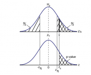
Both decision rules will result in the same decision and it is a matter of preference which one is used.

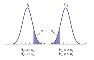
One and Two-tailed Tests

The claim would be in the alternative hypothesis. The burden of proof in hypothesis testing is carried in the alternative. This is because failing to reject the null, the status quo, must be accomplished with 90 or 95 percent significance that it cannot be maintained. Said another way, we want to have only a 5 or 10 percent probability of making a Type I error, rejecting a good null; overthrowing the status quo.

Figure 5 shows the two possible cases and the form of the null and alternative hypothesis that give rise to them.

Effects of Sample Size on Test Statistic

Table 3 summarizes test statistics for varying sample sizes and population standard deviation known and unknown.

A Systematic Approach for Testing A Hypothesis

A systematic approach to hypothesis testing follows the following steps and in this order. This template will work for all hypotheses that you will ever test.

• Set up the null and alternative hypothesis. This is typically the hardest part of the process. Here the question being asked is reviewed. What parameter is being tested, a mean, a proportion, differences in means, etc. Is this a one-tailed test or two-tailed test? Remember, if someone is making a claim it will always be a one-tailed test.
• Decide the level of significance required for this particular case and determine the critical value. These can be found in the appropriate statistical table. The levels of confidence typical for the social sciences are 90, 95 and 99. However, the level of significance is a policy decision and should be based upon the risk of making a Type I error, rejecting a good null. Consider the consequences of making a Type I error.
• Take a sample(s) and calculate the relevant parameters: sample mean, standard deviation, or proportion. Using the formula for the test statistic from above in step 2, now calculate the test statistic for this particular case using the parameters you have just calculated.
• Compare the calculated test statistic and the critical value. Marking these on the graph will give a good visual picture of the situation. There are now only two situations:

a.     The test statistic is in the tail: Cannot Accept the null, the probability that this sample mean (proportion) came from the hypothesized distribution is too small to believe that it is the real home of these sample data.

b.   The test statistic is not in the tail: Cannot Reject the null, the sample data are compatible with the hypothesized population parameter.

• Reach a conclusion. It is best to articulate the conclusion two different ways. First a formal statistical conclusion such as “With a 95 % level of significance we cannot accept the null hypotheses that the population mean is equal to XX (units of measurement)”. The second statement of the conclusion is less formal and states the action, or lack of action, required. If the formal conclusion was that above, then the informal one might be, “The machine is broken and we need to shut it down and call for repairs”.

All hypotheses tested will go through this same process. The only changes are the relevant formulas and those are determined by the hypothesis required to answer the original question.

Full Hypothesis Test Examples

Tests on means.

Jeffrey, as an eight-year old, established a mean time of 16.43 seconds for swimming the 25-yard freestyle, with a standard deviation of 0.8 seconds . His dad, Frank, thought that Jeffrey could swim the 25-yard freestyle faster using goggles. Frank bought Jeffrey a new pair of expensive goggles and timed Jeffrey for 15 25-yard freestyle swims . For the 15 swims, Jeffrey’s mean time was 16 seconds. Frank thought that the goggles helped Jeffrey to swim faster than the 16.43 seconds. Conduct a hypothesis test using a preset α = 0.05.

Solution – Example 6

Set up the Hypothesis Test:

Since the problem is about a mean, this is a test of a single population mean . Set the null and alternative hypothesis:

In this case there is an implied challenge or claim. This is that the goggles will reduce the swimming time. The effect of this is to set the hypothesis as a one-tailed test. The claim will always be in the alternative hypothesis because the burden of proof always lies with the alternative. Remember that the status quo must be defeated with a high degree of confidence, in this case 95 % confidence. The null and alternative hypotheses are thus:

For Jeffrey to swim faster, his time will be less than 16.43 seconds. The “<” tells you this is left-tailed. Determine the distribution needed:

Distribution for the test statistic:

The sample size is less than 30 and we do not know the population standard deviation so this is a t-test and the proper formula is:

Our step 2, setting the level of significance, has already been determined by the problem, .05 for a 95 % significance level. It is worth thinking about the meaning of this choice. The Type I error is to conclude that Jeffrey swims the 25-yard freestyle, on average, in less than 16.43 seconds when, in fact, he actually swims the 25-yard freestyle, on average, in 16.43 seconds. (Reject the null hypothesis when the null hypothesis is true.) For this case the only concern with a Type I error would seem to be that Jeffery’s dad may fail to bet on his son’s victory because he does not have appropriate confidence in the effect of the goggles.

To find the critical value we need to select the appropriate test statistic. We have concluded that this is a t-test on the basis of the sample size and that we are interested in a population mean. We can now draw the graph of the t-distribution and mark the critical value (Figure 6). For this problem the degrees of freedom are n-1, or 14. Looking up 14 degrees of freedom at the 0.05 column of the t-table we find 1.761. This is the critical value and we can put this on our graph.

Step 3 is the calculation of the test statistic using the formula we have selected.

We find that the calculated test statistic is 2.08, meaning that the sample mean is 2.08 standard deviations away from the hypothesized mean of 16.43.

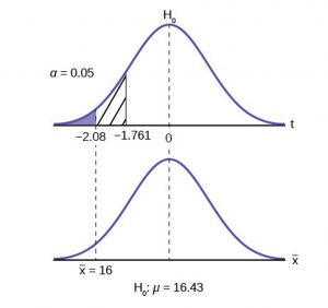
Step 4 has us compare the test statistic and the critical value and mark these on the graph. We see that the test statistic is in the tail and thus we move to step 4 and reach a conclusion. The probability that an average time of 16 minutes could come from a distribution with a population mean of 16.43 minutes is too unlikely for us to accept the null hypothesis. We cannot accept the null.

Step 5 has us state our conclusions first formally and then less formally. A formal conclusion would be stated as: “With a 95% level of significance we cannot accept the null hypothesis that the swimming time with goggles comes from a distribution with a population mean time of 16.43 minutes.” Less formally, “With 95% significance we believe that the goggles improves swimming speed”

If we wished to use the p-value system of reaching a conclusion we would calculate the statistic and take the additional step to find the probability of being 2.08 standard deviations from the mean on a t-distribution. This value is .0187. Comparing this to the α-level of .05 we see that we cannot accept the null. The p-value has been put on the graph as the shaded area beyond -2.08 and it shows that it is smaller than the hatched area which is the alpha level of 0.05. Both methods reach the same conclusion that we cannot accept the null hypothesis.

Jane has just begun her new job as on the sales force of a very competitive company. In a sample of 16 sales calls it was found that she closed the contract for an average value of $108 with a standard deviation of 12 dollars. Test at 5% significance that the population mean is at least $100 against the alternative that it is less than 100 dollars. Company policy requires that new members of the sales force must exceed an average of $100 per contract during the trial employment period. Can we conclude that Jane has met this requirement at the significance level of 95%?

Solution – Example 7

STEP 1 : Set the Null and Alternative Hypothesis.

STEP 2 : Decide the level of significance and draw the graph (Figure 7) showing the critical value.

STEP 3 : Calculate sample parameters and the test statistic.

STEP 4 : Compare test statistic and the critical values

STEP 5 : Reach a Conclusion

The test statistic is a Student’s t because the sample size is below 30; therefore, we cannot use the normal distribution. Comparing the calculated value of the test statistic and the critical value of t ( t a ) at a 5% significance level, we see that the calculated value is in the tail of the distribution. Thus, we conclude that 108 dollars per contract is significantly larger than the hypothesized value of 100 and thus we cannot accept the null hypothesis. There is evidence that supports Jane’s performance meets company standards.

Again we will follow the steps in our analysis of this problem.

Solution – Example 8

STEP 1 : Set the Null and Alternative Hypothesis. The random variable is the quantity of fluid placed in the bottles. This is a continuous random variable and the parameter we are interested in is the mean. Our hypothesis therefore is about the mean. In this case we are concerned that the machine is not filling properly. From what we are told it does not matter if the machine is over-filling or under-filling, both seem to be an equally bad error. This tells us that this is a two-tailed test: if the machine is malfunctioning it will be shutdown regardless if it is from over-filling or under-filling. The null and alternative hypotheses are thus:

STEP 2 : Decide the level of significance and draw the graph showing the critical value.

This problem has already set the level of significance at 99%. The decision seems an appropriate one and shows the thought process when setting the significance level. Management wants to be very certain, as certain as probability will allow, that they are not shutting down a machine that is not in need of repair. To draw the distribution and the critical value, we need to know which distribution to use. Because this is a continuous random variable and we are interested in the mean, and the sample size is greater than 30, the appropriate distribution is the normal distribution and the relevant critical value is 2.575 from the normal table or the t-table at 0.005 column and infinite degrees of freedom. We draw the graph and mark these points (Figure 8).

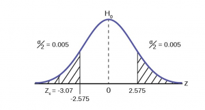
STEP 3 : Calculate sample parameters and the test statistic. The sample parameters are provided, the sample mean is 7.91 and the sample variance is .03 and the sample size is 35. We need to note that the sample variance was provided not the sample standard deviation, which is what we need for the formula. Remembering that the standard deviation is simply the square root of the variance, we therefore know the sample standard deviation, s, is 0.173. With this information we calculate the test statistic as -3.07, and mark it on the graph.

STEP 4 : Compare test statistic and the critical values Now we compare the test statistic and the critical value by placing the test statistic on the graph. We see that the test statistic is in the tail, decidedly greater than the critical value of 2.575. We note that even the very small difference between the hypothesized value and the sample value is still a large number of standard deviations. The sample mean is only 0.08 ounces different from the required level of 8 ounces, but it is 3 plus standard deviations away and thus we cannot accept the null hypothesis.

Three standard deviations of a test statistic will guarantee that the test will fail. The probability that anything is within three standard deviations is almost zero. Actually it is 0.0026 on the normal distribution, which is certainly almost zero in a practical sense. Our formal conclusion would be “ At a 99% level of significance we cannot accept the hypothesis that the sample mean came from a distribution with a mean of 8 ounces” Or less formally, and getting to the point, “At a 99% level of significance we conclude that the machine is under filling the bottles and is in need of repair”.

Media Attributions

• Type1Type2Error
• HypTestFig2
• HypTestFig3
• HypTestPValue
• OneTailTestFig5
• HypTestExam7
• HypTestExam8

Quantitative Analysis for Business Copyright © by Margo Bergman is licensed under a Creative Commons Attribution-NonCommercial-ShareAlike 4.0 International License , except where otherwise noted.

Share This Book

Have a language expert improve your writing

Run a free plagiarism check in 10 minutes, generate accurate citations for free.

• Knowledge Base

Hypothesis Testing | A Step-by-Step Guide with Easy Examples

Published on November 8, 2019 by Rebecca Bevans . Revised on June 22, 2023.

Hypothesis testing is a formal procedure for investigating our ideas about the world using statistics . It is most often used by scientists to test specific predictions, called hypotheses, that arise from theories.

There are 5 main steps in hypothesis testing:

• State your research hypothesis as a null hypothesis and alternate hypothesis (H o ) and (H a  or H 1 ).
• Collect data in a way designed to test the hypothesis.
• Perform an appropriate statistical test .
• Decide whether to reject or fail to reject your null hypothesis.
• Present the findings in your results and discussion section.

Though the specific details might vary, the procedure you will use when testing a hypothesis will always follow some version of these steps.

Table of contents

Step 1: state your null and alternate hypothesis, step 2: collect data, step 3: perform a statistical test, step 4: decide whether to reject or fail to reject your null hypothesis, step 5: present your findings, other interesting articles, frequently asked questions about hypothesis testing.

After developing your initial research hypothesis (the prediction that you want to investigate), it is important to restate it as a null (H o ) and alternate (H a ) hypothesis so that you can test it mathematically.

The alternate hypothesis is usually your initial hypothesis that predicts a relationship between variables. The null hypothesis is a prediction of no relationship between the variables you are interested in.

• H 0 : Men are, on average, not taller than women. H a : Men are, on average, taller than women.

Prevent plagiarism. Run a free check.

For a statistical test to be valid , it is important to perform sampling and collect data in a way that is designed to test your hypothesis. If your data are not representative, then you cannot make statistical inferences about the population you are interested in.

There are a variety of statistical tests available, but they are all based on the comparison of within-group variance (how spread out the data is within a category) versus between-group variance (how different the categories are from one another).

If the between-group variance is large enough that there is little or no overlap between groups, then your statistical test will reflect that by showing a low p -value . This means it is unlikely that the differences between these groups came about by chance.

Alternatively, if there is high within-group variance and low between-group variance, then your statistical test will reflect that with a high p -value. This means it is likely that any difference you measure between groups is due to chance.

Your choice of statistical test will be based on the type of variables and the level of measurement of your collected data .

• an estimate of the difference in average height between the two groups.
• a p -value showing how likely you are to see this difference if the null hypothesis of no difference is true.

Based on the outcome of your statistical test, you will have to decide whether to reject or fail to reject your null hypothesis.

In most cases you will use the p -value generated by your statistical test to guide your decision. And in most cases, your predetermined level of significance for rejecting the null hypothesis will be 0.05 – that is, when there is a less than 5% chance that you would see these results if the null hypothesis were true.

In some cases, researchers choose a more conservative level of significance, such as 0.01 (1%). This minimizes the risk of incorrectly rejecting the null hypothesis ( Type I error ).

The results of hypothesis testing will be presented in the results and discussion sections of your research paper , dissertation or thesis .

In the results section you should give a brief summary of the data and a summary of the results of your statistical test (for example, the estimated difference between group means and associated p -value). In the discussion , you can discuss whether your initial hypothesis was supported by your results or not.

In the formal language of hypothesis testing, we talk about rejecting or failing to reject the null hypothesis. You will probably be asked to do this in your statistics assignments.

However, when presenting research results in academic papers we rarely talk this way. Instead, we go back to our alternate hypothesis (in this case, the hypothesis that men are on average taller than women) and state whether the result of our test did or did not support the alternate hypothesis.

If your null hypothesis was rejected, this result is interpreted as “supported the alternate hypothesis.”

These are superficial differences; you can see that they mean the same thing.

You might notice that we don’t say that we reject or fail to reject the alternate hypothesis . This is because hypothesis testing is not designed to prove or disprove anything. It is only designed to test whether a pattern we measure could have arisen spuriously, or by chance.

If we reject the null hypothesis based on our research (i.e., we find that it is unlikely that the pattern arose by chance), then we can say our test lends support to our hypothesis . But if the pattern does not pass our decision rule, meaning that it could have arisen by chance, then we say the test is inconsistent with our hypothesis .

If you want to know more about statistics , methodology , or research bias , make sure to check out some of our other articles with explanations and examples.

• Normal distribution
• Descriptive statistics
• Measures of central tendency
• Correlation coefficient

Methodology

• Cluster sampling
• Stratified sampling
• Types of interviews
• Cohort study
• Thematic analysis

Research bias

• Implicit bias
• Cognitive bias
• Survivorship bias
• Availability heuristic
• Nonresponse bias
• Regression to the mean

Hypothesis testing is a formal procedure for investigating our ideas about the world using statistics. It is used by scientists to test specific predictions, called hypotheses , by calculating how likely it is that a pattern or relationship between variables could have arisen by chance.

A hypothesis states your predictions about what your research will find. It is a tentative answer to your research question that has not yet been tested. For some research projects, you might have to write several hypotheses that address different aspects of your research question.

A hypothesis is not just a guess — it should be based on existing theories and knowledge. It also has to be testable, which means you can support or refute it through scientific research methods (such as experiments, observations and statistical analysis of data).

Null and alternative hypotheses are used in statistical hypothesis testing . The null hypothesis of a test always predicts no effect or no relationship between variables, while the alternative hypothesis states your research prediction of an effect or relationship.

Cite this Scribbr article

If you want to cite this source, you can copy and paste the citation or click the “Cite this Scribbr article” button to automatically add the citation to our free Citation Generator.

Bevans, R. (2023, June 22). Hypothesis Testing | A Step-by-Step Guide with Easy Examples. Scribbr. Retrieved April 15, 2024, from https://www.scribbr.com/statistics/hypothesis-testing/

Is this article helpful?

Rebecca Bevans

Other students also liked, choosing the right statistical test | types & examples, understanding p values | definition and examples, what is your plagiarism score.

User Preferences

Content preview.

Arcu felis bibendum ut tristique et egestas quis:

• Ut enim ad minim veniam, quis nostrud exercitation ullamco laboris
• Duis aute irure dolor in reprehenderit in voluptate
• Excepteur sint occaecat cupidatat non proident

Keyboard Shortcuts

5.3 - hypothesis testing for one-sample mean.

In the previous section, we learned how to perform a hypothesis test for one proportion. The concepts of hypothesis testing remain constant for any hypothesis test. In these next few sections, we will present the hypothesis test for one mean. We start with our knowledge of the sampling distribution of the sample mean.

Hypothesis Test for One-Sample Mean Section  

Recall that under certain conditions, the sampling distribution of the sample mean, \(\bar{x} \), is approximately normal with mean, \(\mu \), standard error \(\dfrac{\sigma}{\sqrt{n}} \), and estimated standard error \(\dfrac{s}{\sqrt{n}} \).

\(H_0\colon \mu=\mu_0\)

Conditions:

• The distribution of the population is Normal
• The sample size is large \( n>30 \).

Test Statistic:

If at least one of conditions are satisfied, then...

\( t=\dfrac{\bar{x}-\mu_0}{\frac{s}{\sqrt{n}}} \)

will follow a t-distribution with \(n-1 \) degrees of freedom.

Notice when working with continuous data we are going to use a t statistic as opposed to the z statistic. This is due to the fact that the sample size impacts the sampling distribution and needs to be taken into account. We do this by recognizing “degrees of freedom”. We will not go into too much detail about degrees of freedom in this course.

Let’s look at an example.

Example 5-1 Section  

This depends on the standard deviation of \(\bar{x} \) . 

\begin{align} t^*&=\dfrac{\bar{x}-\mu}{\frac{s}{\sqrt{n}}}\\&=\dfrac{8.3-8.5}{\frac{1.2}{\sqrt{61}}}\\&=-1.3 \end{align} 

Thus, we are asking if \(-1.3\) is very far away from zero, since that corresponds to the case when \(\bar{x}\) is equal to \(\mu_0 \). If it is far away, then it is unlikely that the null hypothesis is true and one rejects it. Otherwise, one cannot reject the null hypothesis. 

Statistics Made Easy

One Sample t-test: Definition, Formula, and Example

A  one sample t-test  is used to test whether or not the mean of a population is equal to some value.

This tutorial explains the following:

• The motivation for performing a one sample t-test.
• The formula to perform a one sample t-test.
• The assumptions that should be met to perform a one sample t-test.
• An example of how to perform a one sample t-test.

One Sample t-test: Motivation

Suppose we want to know whether or not the mean weight of a certain species of turtle in Florida is equal to 310 pounds. Since there are thousands of turtles in Florida, it would be extremely time-consuming and costly to go around and weigh each individual turtle.

Instead, we might take a simple random sample of 40 turtles and use the mean weight of the turtles in this sample to estimate the true population mean:

However, it’s virtually guaranteed that the mean weight of turtles in our sample will differ from 310 pounds. The question is whether or not this difference is statistically significant . Fortunately, a one sample t-test allows us to answer this question.

One Sample t-test: Formula

A one-sample t-test always uses the following null hypothesis:

• H 0 :  μ = μ 0 (population mean is equal to some hypothesized value μ 0 )

The alternative hypothesis can be either two-tailed, left-tailed, or right-tailed:

• H 1 (two-tailed):  μ ≠ μ 0 (population mean is not equal to some hypothesized value μ 0 )
• H 1 (left-tailed):  μ < μ 0 (population mean is less than some hypothesized value μ 0 )
• H 1 (right-tailed):  μ > μ 0 (population mean is greater than some hypothesized value μ 0 )

We use the following formula to calculate the test statistic t:

t = ( x  – μ) / (s/√ n )

• x : sample mean
• μ 0 : hypothesized population mean
• s:  sample standard deviation
• n:  sample size

If the p-value that corresponds to the test statistic t with (n-1) degrees of freedom is less than your chosen significance level (common choices are 0.10, 0.05, and 0.01) then you can reject the null hypothesis.

One Sample t-test: Assumptions

For the results of a one sample t-test to be valid, the following assumptions should be met:

• The variable under study should be either an interval or ratio variable .
• The observations in the sample should be independent .
• The variable under study should be approximately normally distributed.  You can check this assumption by creating a histogram and visually checking if the distribution has roughly a “bell shape.”
• The variable under study should have no outliers. You can check this assumption by creating a boxplot and visually checking for outliers.

One Sample t-test : Example

Suppose we want to know whether or not the mean weight of a certain species of turtle is equal to 310 pounds. To test this, will perform a one-sample t-test at significance level α = 0.05 using the following steps:

Step 1: Gather the sample data.

Suppose  we collect a random sample of turtles with the following information:

• Sample size n = 40
• Sample mean weight  x  = 300
• Sample standard deviation s = 18.5

Step 2: Define the hypotheses.

We will perform the one sample t-test with the following hypotheses:

• H 0 :  μ = 310 (population mean is equal to 310 pounds)
• H 1 :  μ ≠ 310 (population mean is not equal to 310 pounds)

Step 3: Calculate the test statistic  t .

t = ( x  – μ) / (s/√ n ) = (300-310) / (18.5/√ 40 ) =  -3.4187

Step 4: Calculate the p-value of the test statistic  t .

According to the T Score to P Value Calculator , the p-value associated with t = -3.4817 and degrees of freedom = n-1 = 40-1 = 39 is  0.00149 .

Step 5: Draw a conclusion.

Since this p-value is less than our significance level α = 0.05, we reject the null hypothesis. We have sufficient evidence to say that the mean weight of this species of turtle is not equal to 310 pounds.

Note:  You can also perform this entire one sample t-test by simply using the One Sample t-test calculator .

Additional Resources

The following tutorials explain how to perform a one-sample t-test using different statistical programs:

How to Perform a One Sample t-test in Excel How to Perform a One Sample t-test in SPSS How to Perform a One Sample t-test in Stata How to Perform a One Sample t-test in R How to Conduct a One Sample t-test in Python How to Perform a One Sample t-test on a TI-84 Calculator

Published by Zach

Leave a reply cancel reply.

Your email address will not be published. Required fields are marked *

• school Campus Bookshelves
• menu_book Bookshelves
• perm_media Learning Objects
• login Login
• how_to_reg Request Instructor Account
• hub Instructor Commons
• Download Page (PDF)
• Download Full Book (PDF)
• Periodic Table
• Physics Constants
• Scientific Calculator
• Reference & Cite
• Tools expand_more
• Readability

selected template will load here

This action is not available.

11: Hypothesis Testing with One Sample

• Last updated
• Save as PDF
• Page ID 19096

One job of a statistician is to make statistical inferences about populations based on samples taken from the population. Confidence intervals are one way to estimate a population parameter. Another way to make a statistical inference is to make a decision about a parameter. For instance, a car dealer advertises that its new small truck gets 35 miles per gallon, on average. A tutoring service claims that its method of tutoring helps 90% of its students get an A or a B. A company says that women managers in their company earn an average of $60,000 per year.

• 11.1: Prelude to Hypothesis Testing A statistician will make a decision about claims via a process called "hypothesis testing." A hypothesis test involves collecting data from a sample and evaluating the data. Then, the statistician makes a decision as to whether or not there is sufficient evidence, based upon analysis of the data, to reject the null hypothesis.
• Null and Alternative Hypotheses (Exercises)
• Outcomes and the Type I and Type II Errors (Exercises)
• Distribution Needed for Hypothesis Testing (Exercises)
• Rare Events, the Sample, Decision and Conclusion (Exercises)
• 11.6: Additional Information and Full Hypothesis Test Examples The hypothesis test itself has an established process. This can be summarized as follows: Determine H0 and Ha. Remember, they are contradictory. Determine the random variable. Determine the distribution for the test. Draw a graph, calculate the test statistic, and use the test statistic to calculate the p-value. (A z-score and a t-score are examples of test statistics.) Compare the preconceived α with the p-value, make a decision (reject or do not reject H0), and write a clear conclusion.
• 11.7: Hypothesis Testing of a Single Mean and Single Proportion (Worksheet) A statistics Worksheet:  The student will select the appropriate distributions to use in each case. The student will conduct hypothesis tests and interpret the results.
• 11.8: Hypothesis Testing with One Sample (Exercises) These are homework exercises to accompany the Textmap created for "Introductory Statistics" by OpenStax.

Contributors

• Template:ContribOpenStax

An open portfolio of interoperable, industry leading products

The Dotmatics digital science platform provides the first true end-to-end solution for scientific R&D, combining an enterprise data platform with the most widely used applications for data analysis, biologics, flow cytometry, chemicals innovation, and more.

Statistical analysis and graphing software for scientists

Bioinformatics, cloning, and antibody discovery software

Plan, visualize, & document core molecular biology procedures

Electronic Lab Notebook to organize, search and share data

Proteomics software for analysis of mass spec data

Modern cytometry analysis platform

Analysis, statistics, graphing and reporting of flow cytometry data

Software to optimize designs of clinical trials

• One sample t test

A one sample t test compares the mean with a hypothetical value. In most cases, the hypothetical value comes from theory. For example, if you express your data as 'percent of control', you can test whether the average differs significantly from 100. The hypothetical value can also come from previous data. For example, compare whether the mean systolic blood pressure differs from 135, a value determined in a previous study.

1. Choose data entry format

Caution: Changing format will erase your data.

2. Specify the hypothetical mean value

3. enter data, 4. view the results, learn more about the one sample t test.

In this article you will learn the requirements and assumptions of a one sample t test, how to format and interpret the results of a one sample t test, and when to use different types of t tests.

One sample t test: Overview

The one sample t test, also referred to as a single sample t test, is a statistical hypothesis test used to determine whether the mean calculated from sample data collected from a single group is different from a designated value specified by the researcher. This designated value does not come from the data itself, but is an external value chosen for scientific reasons. Often, this designated value is a mean previously established in a population, a standard value of interest, or a mean concluded from other studies. Like all hypothesis testing, the one sample t test determines if there is enough evidence reject the null hypothesis (H0) in favor of an alternative hypothesis (H1). The null hypothesis for a one sample t test can be stated as: "The population mean equals the specified mean value." The alternative hypothesis for a one sample t test can be stated as: "The population mean is different from the specified mean value."

The one sample t test differs from most statistical hypothesis tests because it does not compare two separate groups or look at a relationship between two variables. It is a straightforward comparison between data gathered on a single variable from one population and a specified value defined by the researcher. The one sample t test can be used to look for a difference in only one direction from the standard value (a one-tailed t test ) or can be used to look for a difference in either direction from the standard value (a two-tailed t test ).

Requirements and Assumptions for a one sample t test

A one sample t test should be used only when data has been collected on one variable for a single population and there is no comparison being made between groups. For a valid one sample t test analysis, data values must be all of the following:

The one sample t test assumes that all "errors" in the data are independent. The term "error" refers to the difference between each value and the group mean. The results of a t test only make sense when the scatter is random - that whatever factor caused a value to be too high or too low affects only that one value. Prism cannot test this assumption, but there are graphical ways to explore data to verify this assumption is met.

A t test is only appropriate to apply in situations where data represent variables that are continuous measurements. As they rely on the calculation of a mean value, variables that are categorical should not be analyzed using a t test.

The results of a t test should be based on a random sample and only be generalized to the larger population from which samples were drawn.

As with all parametric hypothesis testing, the one sample t test assumes that you have sampled your data from a population that follows a normal (or Gaussian) distribution. While this assumption is not as important with large samples, it is important with small sample sizes, especially less than 10. If your data do not come from a Gaussian distribution , there are three options to accommodate this. One option is to transform the values to make the distribution more Gaussian, perhaps by transforming all values to their reciprocals or logarithms. Another choice is to use the Wilcoxon signed rank nonparametric test instead of the t test. A final option is to use the t test anyway, knowing that the t test is fairly robust to departures from a Gaussian distribution with large samples.

How to format a one sample t test

Ideally, data for a one sample t test should be collected and entered as a single column from which a mean value can be easily calculated. If data is entered on a table with multiple subcolumns, Prism requires one of the following choices to be selected to perform the analysis:

• Each subcolumn of data can be analyzed separately
• An average of the values in the columns across each row can be calculated, and the analysis conducted on this new stack of means, or
• All values in all columns can be treated as one sample of data (paying no attention to which row or column any values are in).

How the one sample t test calculator works

Prism calculates the t ratio by dividing the difference between the actual and hypothetical means by the standard error of the actual mean. The equation is written as follows, where x is the calculated mean, μ is the hypothetical mean (specified value), S is the standard deviation of the sample, and n is the sample size:

A p value is computed based on the calculated t ratio and the numbers of degrees of freedom present (which equals sample size minus 1). The one sample t test calculator assumes it is a two-tailed one sample t test, meaning you are testing for a difference in either direction from the specified value.

How to interpret results of a one sample t test

As discussed, a one sample t test compares the mean of a single column of numbers against a hypothetical mean. This hypothetical mean can be based upon a specific standard or other external prediction. The test produces a P value which requires careful interpretation.

The p value answers this question: If the data were sampled from a Gaussian population with a mean equal to the hypothetical value you entered, what is the chance of randomly selecting N data points and finding a mean as far (or further) from the hypothetical value as observed here?

If the p value is large (usually defined to mean greater than 0.05), the data do not give you any reason to conclude that the population mean differs from the designated value to which it has been compared. This is not the same as saying that the true mean equals the hypothetical value, but rather states that there is no evidence of a difference. Thus, we cannot reject the null hypothesis (H0).

If the p value is small (usually defined to mean less than or equal to 0.05), then it is unlikely that the discrepancy observed between the sample mean and hypothetical mean is due to a coincidence arising from random sampling. There is evidence to reject the idea that the difference is coincidental and conclude instead that the population has a mean that is different from the hypothetical value to which it has been compared. The difference is statistically significant, and the null hypothesis is therefore rejected.

If the null hypothesis is rejected, the question of whether the difference is scientifically important still remains. The confidence interval can be a useful tool in answering this question. Prism reports the 95% confidence interval for the difference between the actual and hypothetical mean. In interpreting these results, one can be 95% sure that this range includes the true difference. It requires scientific judgment to determine if this difference is truly meaningful.

Performing t tests? We can help.

Sign up for more information on how to perform t tests and other common statistical analyses.

When to use different types of t tests

There are three types of t tests which can be used for hypothesis testing:

• Independent two-sample (or unpaired) t test
• Paired sample t test

As described, a one sample t test should be used only when data has been collected on one variable for a single population and there is no comparison being made between groups. It only applies when the mean value for data is intended to be compared to a fixed and defined number.

In most cases involving data analysis, however, there are multiple groups of data either representing different populations being compared, or the same population being compared at different times or conditions. For these situations, it is not appropriate to use a one sample t test. Other types of t tests are appropriate for these specific circumstances:

Independent Two-Sample t test (Unpaired t test)

The independent sample t test, also referred to as the unpaired t test, is used to compare the means of two different samples. The independent two-sample t test comes in two different forms:

• the standard Student's t test, which assumes that the variance of the two groups are equal.
• the Welch's t test , which is less restrictive compared to the original Student's test. This is the test where you do not assume that the variance is the same in the two groups, which results in fractional degrees of freedom.

The two methods give very similar results when the sample sizes are equal and the variances are similar.

Paired Sample t test

The paired sample t test is used to compare the means of two related groups of samples. Put into other words, it is used in a situation where you have two values (i.e., a pair of values) for the same group of samples. Often these two values are measured from the same samples either at two different times, under two different conditions, or after a specific intervention.

You can perform multiple independent two-sample comparison tests simultaneously in Prism. Select from parametric and nonparametric tests and specify if the data are unpaired or paired. Try performing a t test with a 30-day free trial of Prism .

Watch this video to learn how to choose between a paired and unpaired t test.

Example of how to apply the appropriate t test

"Alkaline" labeled bottled drinking water has become fashionable over the past several years. Imagine we have collected a random sample of 30 bottles of "alkaline" drinking water from a number of different stores to represent the population of "alkaline" bottled water for a particular brand available to the general consumer. The labels on each of the bottles claim that the pH of the "alkaline" water is 8.5. A laboratory then proceeds to measure the exact pH of the water in each bottle.

Table 1: pH of water in random sample of "alkaline bottled water"

If you look at the table above, you see that some bottles have a pH measured to be lower than 8.5, while other bottles have a pH measured to be higher. What can the data tell us about the actual pH levels found in this brand of "alkaline" water bottles marketed to the public as having a pH of 8.5? Statistical hypothesis testing provides a sound method to evaluate this question. Which specific test to use, however, depends on the specific question being asked.

Is a t test appropriate to apply to this data?

Let's start by asking: Is a t test an appropriate method to analyze this set of pH data? The following list reviews the requirements and assumptions for using a t test:

• Independent sampling : In an independent sample t test, the data values are independent. The pH of one bottle of water does not depend on the pH of any other water bottle. (An example of dependent values would be if you collected water bottles from a single production lot. A sample from a single lot is representative only of that lot, not of alkaline bottled water in general).
• Continuous variable : The data values are pH levels, which are numerical measurements that are continuous.
• Random sample : We assume the water bottles are a simple random sample from the population of "alkaline" water bottles produced by this brand as they are a mix of many production lots.
• Normal distribution : We assume the population from which we collected our samples has pH levels that are normally distributed. To verify this, we should visualize the data graphically. The figure below shows a histogram for the pH measurements of the water bottles. From a quick look at the histogram, we see that there are no unusual points, or outliers. The data look roughly bell-shaped, so our assumption of a normal distribution seems reasonable. The QQ plot can also be used to graphically assess normality and is the preferred choice when the sample size is small.

Based upon these features and assumptions being met, we can conclude that a t test is an appropriate method to be applied to this set of data.

Which t test is appropriate to use?

The next decision is which t test to apply, and this depends on the exact question we would like our analysis to answer. This example illustrates how each type of t test could be chosen for a specific analysis, and why the one sample t test is the correct choice to determine if the measured pH of the bottled water samples match the advertised pH of 8.5.

We could be interested in determining whether a certain characteristic of a water bottle is associated with having a higher or lower pH, such as whether bottles are glass or plastic. For this questions, we would effectively be dividing the bottles into 2 separate groups and comparing the means of the pH between the 2 groups. For this analysis, we would elect to use a two sample t test because we are comparing the means of two independent groups.

We could also be interested in learning if pH is affected by a water bottle being opened and exposed to the air for a week. In this case, each original sample would be tested for pH level after a week had elapsed and the water had been exposed to the air, creating a second set of sample data. To evaluate whether this exposure affected pH, we would again be comparing two different groups of data, but this time the data are in paired samples each having an original pH measurement and a second measurement from after the week of exposure to the open air. For this analysis, it is appropriate to use a paired t test so that data for each bottle is assembled in rows, and the change in pH is considered bottle by bottle.

Returning to the original question we set out to answer-whether bottled water that is advertised to have a pH of 8.5 actually meets this claim-it is now clear that neither an independent two sample t test or a paired t test would be appropriate. In this case, all 30 pH measurements are sampled from one group representing bottled drinking water labeled "alkaline" available to the general consumer. We wish to compare this measured mean with an expected advertised value of 8.5. This is the exact situation for which one should employ a one sample t test!

From a quick look at the descriptive statistics, we see that the mean of the sample measurements is 8.513, slightly above 8.5. Does this average from our sample of 30 bottles validate the advertised claim of pH 8.5? By applying Prism's one sample t test analysis to this data set, we will get results by which we can evaluate whether the null hypothesis (that there is no difference between the mean pH level in the water bottles and the pH level advertised on the bottles) should be accepted or rejected.

How to Perform a One Sample T Test in Prism

In prior versions of Prism, the one sample t test and the Wilcoxon rank sum tests were computed as part of Prism's Column Statistics analysis. Now, starting with Prism 8, performing one sample t tests is even easier with a separate analysis in Prism.

Steps to perform a one sample t test in Prism

• Create a Column data table.
• Enter each data set in a single Y column so all values from each group are stacked into a column. Prism will perform a one sample t test (or Wilcoxon rank sum test) on each column you enter.
• Click Analyze, look in the list of Column analyses, and choose one sample t test and Wilcoxon test.

It's that simple! Prism streamlines your t test analysis so you can make more accurate and more informed data interpretations. Start your 30-day free trial of Prism and try performing your first one sample t test in Prism.

Watch this video for a step-by-step tutorial on how to perform a t test in Prism.

We Recommend:

Analyze, graph and present your scientific work easily with GraphPad Prism. No coding required.

• school Campus Bookshelves
• menu_book Bookshelves
• perm_media Learning Objects
• login Login
• how_to_reg Request Instructor Account
• hub Instructor Commons
• Download Page (PDF)
• Download Full Book (PDF)
• Periodic Table
• Physics Constants
• Scientific Calculator
• Reference & Cite
• Tools expand_more
• Readability

selected template will load here

This action is not available.

9: Hypothesis Testing with One Sample

• Last updated
• Save as PDF
• Page ID 113345

One job of a statistician is to make statistical inferences about populations based on samples taken from the population. Confidence intervals are one way to estimate a population parameter. Another way to make a statistical inference is to make a decision about a parameter. For instance, a car dealer advertises that its new small truck gets 35 miles per gallon, on average. A tutoring service claims that its method of tutoring helps 90% of its students get an A or a B. A company says that women managers in their company earn an average of $60,000 per year.

• 9.0: Prelude to Hypothesis Testing A statistician will make a decision about claims via a process called "hypothesis testing." A hypothesis test involves collecting data from a sample and evaluating the data. Then, the statistician makes a decision as to whether or not there is sufficient evidence, based upon analysis of the data, to reject the null hypothesis.
• 9.1E: Null and Alternative Hypotheses (Exercises)
• 9.2E: Outcomes and the Type I and Type II Errors (Exercises)
• 9.3E: Distribution Needed for Hypothesis Testing (Exercises)
• 9.4E: Rare Events, the Sample, Decision and Conclusion (Exercises)
• 9.5: Additional Information and Full Hypothesis Test Examples The hypothesis test itself has an established process. This can be summarized as follows: Determine H0 and Ha. Remember, they are contradictory. Determine the random variable. Determine the distribution for the test. Draw a graph, calculate the test statistic, and use the test statistic to calculate the p-value. (A z-score and a t-score are examples of test statistics.) Compare the preconceived α with the p-value, make a decision (reject or do not reject H0), and write a clear conclusion.
• 9.6: Hypothesis Testing of a Single Mean and Single Proportion (Worksheet) A statistics Worksheet:  The student will select the appropriate distributions to use in each case. The student will conduct hypothesis tests and interpret the results.
• 9.E: Hypothesis Testing with One Sample (Exercises) These are homework exercises to accompany the Textmap created for "Introductory Statistics" by OpenStax.

• school Campus Bookshelves
• menu_book Bookshelves
• perm_media Learning Objects
• login Login
• how_to_reg Request Instructor Account
• hub Instructor Commons
• Download Page (PDF)
• Download Full Book (PDF)
• Periodic Table
• Physics Constants
• Scientific Calculator
• Reference & Cite
• Tools expand_more
• Readability

selected template will load here

This action is not available.

8.5: Hypothesis Test on a Single Variance

• Last updated
• Save as PDF
• Page ID 25677

A test of a single variance assumes that the underlying distribution is normal . The null and alternative hypotheses are stated in terms of the population variance (or population standard deviation). The test statistic is:

\[\chi^{2} = \frac{(n-1)s^{2}}{\sigma^{2}} \label{test}\]

• \(n\) is the the total number of data
• \(s^{2}\) is the sample variance
• \(\sigma^{2}\) is the population variance

You may think of \(s\) as the random variable in this test. The number of degrees of freedom is \(df = n - 1\). A test of a single variance may be right-tailed, left-tailed, or two-tailed. The next example will show you how to set up the null and alternative hypotheses. The null and alternative hypotheses contain statements about the population variance.

Example 8.5.1

Math instructors are not only interested in how their students do on exams, on average, but how the exam scores vary. To many instructors, the variance (or standard deviation) may be more important than the average.

Suppose a math instructor believes that the standard deviation for his final exam is five points. One of his best students thinks otherwise. The student claims that the standard deviation is more than five points. If the student were to conduct a hypothesis test, what would the null and alternative hypotheses be?

Even though we are given the population standard deviation, we can set up the test using the population variance as follows.

• \(H_{0}: \sigma^{2} = 5^{2}\)
• \(H_{a}: \sigma^{2} > 5^{2}\)

Exercise 8.5.1

A SCUBA instructor wants to record the collective depths each of his students dives during their checkout. He is interested in how the depths vary, even though everyone should have been at the same depth. He believes the standard deviation is three feet. His assistant thinks the standard deviation is less than three feet. If the instructor were to conduct a test, what would the null and alternative hypotheses be?

• \(H_{0}: \sigma^{2} = 3^{2}\)
• \(H_{a}: \sigma^{2} > 3^{2}\)

Example 8.5.2

With individual lines at its various windows, a post office finds that the standard deviation for normally distributed waiting times for customers on Friday afternoon is 7.2 minutes. The post office experiments with a single, main waiting line and finds that for a random sample of 25 customers, the waiting times for customers have a standard deviation of 3.5 minutes.

With a significance level of 5%, test the claim that a single line causes lower variation among waiting times (shorter waiting times) for customers .

Since the claim is that a single line causes less variation, this is a test of a single variance. The parameter is the population variance, \(\sigma^{2}\), or the population standard deviation, \(\sigma\).

Random Variable: The sample standard deviation, \(s\), is the random variable. Let \(s = \text{standard deviation for the waiting times}\).

• \(H_{0}: \sigma^{2} = 7.2^{2}\)
• \(H_{a}: \sigma^{2} < 7.2^{2}\)

The word "less" tells you this is a left-tailed test.

Distribution for the test: \(\chi^{2}_{24}\), where:

• \(n = \text{the number of customers sampled}\)
• \(df = n - 1 = 25 - 1 = 24\)

Calculate the test statistic (Equation \ref{test}):

\[\chi^{2} = \frac{(n-1)s^{2}}{\sigma^{2}} = \frac{(25-1)(3.5)^{2}}{7.2^{2}} = 5.67 \nonumber\]

where \(n = 25\), \(s = 3.5\), and \(\sigma = 7.2\).

Probability statement: \(p\text{-value} = P(\chi^{2} < 5.67) = 0.000042\)

Compare \(\alpha\) and the \(p\text{-value}\) :

\[\alpha = 0.05 (p\text{-value} = 0.000042 \alpha > p\text{-value} \nonumber\]

Make a decision: Since \(\alpha > p\text{-value}\), reject \(H_{0}\). This means that you reject \(\sigma^{2} = 7.2^{2}\). In other words, you do not think the variation in waiting times is 7.2 minutes; you think the variation in waiting times is less.

Conclusion: At a 5% level of significance, from the data, there is sufficient evidence to conclude that a single line causes a lower variation among the waiting times or with a single line, the customer waiting times vary less than 7.2 minutes.

In 2nd DISTR , use 7:χ2cdf . The syntax is (lower, upper, df) for the parameter list. For Example , χ2cdf(-1E99,5.67,24) . The \(p\text{-value} = 0.000042\).

Exercise 8.5.2

The FCC conducts broadband speed tests to measure how much data per second passes between a consumer’s computer and the internet. As of August of 2012, the standard deviation of Internet speeds across Internet Service Providers (ISPs) was 12.2 percent. Suppose a sample of 15 ISPs is taken, and the standard deviation is 13.2. An analyst claims that the standard deviation of speeds is more than what was reported. State the null and alternative hypotheses, compute the degrees of freedom, the test statistic, sketch the graph of the p -value, and draw a conclusion. Test at the 1% significance level.

• \(H_{0}: \sigma^{2} = 12.2^{2}\)
• \(H_{a}: \sigma^{2} > 12.2^{2}\)

In 2nd DISTR , use7: χ2cdf . The syntax is (lower, upper, df) for the parameter list. χ2cdf(16.39,10^99,14) . The \(p\text{-value} = 0.2902\).

\(df = 14\)

\[\text{chi}^{2} \text{test statistic} = 16.39 \nonumber\]

The \(p\text{-value}\) is \(0.2902\), so we decline to reject the null hypothesis. There is not enough evidence to suggest that the variance is greater than \(12.2^{2}\).

• “AppleInsider Price Guides.” Apple Insider, 2013. Available online at http://appleinsider.com/mac_price_guide (accessed May 14, 2013).
• Data from the World Bank, June 5, 2012.

To test variability, use the chi-square test of a single variance. The test may be left-, right-, or two-tailed, and its hypotheses are always expressed in terms of the variance (or standard deviation).

Formula Review

\(\chi^{2} = \frac{(n-1) \cdot s^{2}}{\sigma^{2}}\) Test of a single variance statistic where:

\(n: \text{sample size}\)

\(s: \text{sample standard deviation}\)

\(\sigma: \text{population standard deviation}\)

\(df = n – 1 \text{Degrees of freedom}\)

Test of a Single Variance

• Use the test to determine variation.
• The degrees of freedom is the \(\text{number of samples} - 1\).
• The test statistic is \(\frac{(n-1) \cdot s^{2}}{\sigma^{2}}\), where \(n = \text{the total number of data}\), \(s^{2} = \text{sample variance}\), and \(\sigma^{2} = \text{population variance}\).
• The test may be left-, right-, or two-tailed.

Use the following information to answer the next three exercises: An archer’s standard deviation for his hits is six (data is measured in distance from the center of the target). An observer claims the standard deviation is less.

Exercise 8.5.3

What type of test should be used?

a test of a single variance

Exercise 8.5.4

State the null and alternative hypotheses.

Exercise 8.5.5

Is this a right-tailed, left-tailed, or two-tailed test?

a left-tailed test

Use the following information to answer the next three exercises: The standard deviation of heights for students in a school is 0.81. A random sample of 50 students is taken, and the standard deviation of heights of the sample is 0.96. A researcher in charge of the study believes the standard deviation of heights for the school is greater than 0.81.

Exercise 8.5.6

\(H_{0}: \sigma^{2} = 0.81^{2}\);

\(H_{a}: \sigma^{2} > 0.81^{2}\)

\(df =\) ________

Use the following information to answer the next four exercises: The average waiting time in a doctor’s office varies. The standard deviation of waiting times in a doctor’s office is 3.4 minutes. A random sample of 30 patients in the doctor’s office has a standard deviation of waiting times of 4.1 minutes. One doctor believes the variance of waiting times is greater than originally thought.

Exercise 8.5.7

Exercise 8.5.8.

What is the test statistic?

Exercise 8.5.9

What is the \(p\text{-value}\)?

Exercise 8.5.10

What can you conclude at the 5% significance level?