Reset password New user? Sign up
Existing user? Log in

Linear Models
Already have an account? Log in here.
- Brilliant Mathematics
- Mahindra Jain
A linear model is an equation that describes a relationship between two quantities that show a constant rate of change.
Writing and Using Linear Models
We represent linear relationships graphically with straight lines. A linear model is usually described by two parameters: the slope, often called the growth factor or rate of change, and the \(y\)-intercept, often called the initial value. Given the slope \(m\) and the \(y\)-intercept \(b,\) the linear model can be written as a linear function \(y = mx + b.\)
We can represent the position of a car moving at a constant velocity with a linear model.
In the figure above, the rate of change is \(\frac{200 \text{ m}}{10\text{ s}}, \) or \(20 \text{ m/s},\) so \(m=20.\) The initial value is \(200 \text{ meters}\) so \(b = 200.\) The linear model that represents this car's position is \(y=20x + 200.\)
What is the equation of a line with slope \(4\) and \(y\)-intercept \(6?\)
To write a linear model we need to know both the rate of change and the initial value. Once we have written a linear model, we can use it to solve all types of problems.
A gym has 100 members. The gym plans to increase membership by 10 members every year. Write an equation to represent the relationship between the number of members, \(y,\) and the years from now, \(x.\) Answer The initial value is 100 and the rate of change is 10. Therefore, \(y=10x+100.\)
The table below shows the cost of an ice cream cone \(y\) with \(x\) toppings. Write an equation that models the relationship between \(x\) and \(y.\) Toppings \(x\) Cost \(y\) 2 $3.50 3 $3.75 5 $4.25 Answer Adding one additional topping costs \($3.75-$3.50=$0.25\) or \(\frac{$4.25-$3.75}{2} = $0.25.\) If an ice cream cone with two toppings costs $3.50 each topping costs $0.25, then a cone without any toppings must cost $3.00. Therefore, the rate of change is 0.25, the initial value is 3, and \(y=0.25x + 3.\)
The position \(y\) (in kilometers) of a car at time \(t\) (in hours) is given by \(y = 80t + 300.\) How far does the car travel in one hour? Answer When \(t\) increases by one hour, \(y\) increases by 80 kilometers, so our answer is 80 kilometers. \( _\square \)
Suppose your bank account balance \(y\) (in dollars) after \(t\) years is given by \(y = 10000t + 50000.\) In how many years will you have 100,000 dollars? Answer Plugging 100,000 into \(y\) gives \[\begin{align} 100000 =& 10000t + 50000 \\ 50000 =& 10000t \\ 5 =& t. \end{align}\] Therefore, you need 5 years. \( _\square \)
Henry deposits the same amount of money into his bank account each week. After six weeks of saving money, Henry has $70 in his bank account. After ten weeks of saving money, he has $82. Which equation represents the amount of money \(y\) that Henry has in his bank account after \(x\) weeks?
Problem Loading...
Note Loading...
Set Loading...
Linear Programming
Linear programming is a process that is used to determine the best outcome of a linear function. It is the best method to perform linear optimization by making a few simple assumptions. The linear function is known as the objective function. Real-world relationships can be extremely complicated. However, linear programming can be used to depict such relationships, thus, making it easier to analyze them.
Linear programming is used in many industries such as energy, telecommunication, transportation, and manufacturing. This article sheds light on the various aspects of linear programming such as the definition, formula, methods to solve problems using this technique, and associated linear programming examples.
| 1. | |
| 2. | |
| 3. | |
| 4. | |
| 5. | |
| 6. |
What is Linear Programming?
Linear programming, also abbreviated as LP, is a simple method that is used to depict complicated real-world relationships by using a linear function . The elements in the mathematical model so obtained have a linear relationship with each other. Linear programming is used to perform linear optimization so as to achieve the best outcome.
Linear Programming Definition
Linear programming can be defined as a technique that is used for optimizing a linear function in order to reach the best outcome. This linear function or objective function consists of linear equality and inequality constraints. We obtain the best outcome by minimizing or maximizing the objective function .
Linear Programming Examples
Suppose a postman has to deliver 6 letters in a day from the post office (located at A) to different houses (U, V, W, Y, Z). The distance between the houses is indicated on the lines as given in the image. If the postman wants to find the shortest route that will enable him to deliver the letters as well as save on fuel then it becomes a linear programming problem. Thus, LP will be used to get the optimal solution which will be the shortest route in this example.

Linear Programming Formula
A linear programming problem will consist of decision variables , an objective function, constraints, and non-negative restrictions. The decision variables, x, and y, decide the output of the LP problem and represent the final solution. The objective function, Z, is the linear function that needs to be optimized (maximized or minimized) to get the solution. The constraints are the restrictions that are imposed on the decision variables to limit their value. The decision variables must always have a non-negative value which is given by the non-negative restrictions. The general formula of a linear programming problem is given below:
- Objective Function: Z = ax + by
- Constraints: cx + dy ≤ e, fx + gy ≤ h. The inequalities can also be "≥"
- Non-negative restrictions: x ≥ 0, y ≥ 0
How to Solve Linear Programming Problems?
The most important part of solving linear programming problem is to first formulate the problem using the given data. The steps to solve linear programming problems are given below:
- Step 1: Identify the decision variables.
- Step 2: Formulate the objective function. Check whether the function needs to be minimized or maximized.
- Step 3: Write down the constraints.
- Step 4: Ensure that the decision variables are greater than or equal to 0. (Non-negative restraint)
- Step 5: Solve the linear programming problem using either the simplex or graphical method.
Let us study about these methods in detail in the following sections.
Linear Programming Methods
There are two main methods available for solving linear programming problem. These are the simplex method and the graphical method. Given below are the steps to solve a linear programming problem using both methods.
Linear Programming by Simplex Method
The simplex method in lpp can be applied to problems with two or more decision variables. Suppose the objective function Z = 40\(x_{1}\) + 30\(x_{2}\) needs to be maximized and the constraints are given as follows:
\(x_{1}\) + \(x_{2}\) ≤ 12
2\(x_{1}\) + \(x_{2}\) ≤ 16
\(x_{1}\) ≥ 0, \(x_{2}\) ≥ 0
Step 1: Add another variable, known as the slack variable, to convert the inequalities into equations. Also, rewrite the objective function as an equation .
- 40\(x_{1}\) - 30\(x_{2}\) + Z = 0
\(x_{1}\) + \(x_{2}\) + \(y_{1}\) =12
2\(x_{1}\) + \(x_{2}\) + \(y_{2}\) =16
\(y_{1}\) and \(y_{2}\) are the slack variables.
Step 2: Construct the initial simplex matrix as follows:
\(\begin{bmatrix} x_{1} & x_{2} &y_{1} & y_{2} & Z & \\ 1&1 &1 &0 &0 &12 \\ 2& 1 & 0& 1 & 0 & 16 \\ -40&-30&0&0&1&0 \end{bmatrix}\)
Step 3: Identify the column with the highest negative entry. This is called the pivot column. As -40 is the highest negative entry, thus, column 1 will be the pivot column.
Step 4: Divide the entries in the rightmost column by the entries in the pivot column. We exclude the entries in the bottom-most row.
12 / 1 = 12
The row containing the smallest quotient is identified to get the pivot row. As 8 is the smaller quotient as compared to 12 thus, row 2 becomes the pivot row. The intersection of the pivot row and the pivot column gives the pivot element.
Thus, pivot element = 2.
Step 5: With the help of the pivot element perform pivoting, using matrix properties , to make all other entries in the pivot column 0.
Using the elementary operations divide row 2 by 2 (\(R_{2}\) / 2)
\(\begin{bmatrix} x_{1} & x_{2} &y_{1} & y_{2} & Z & \\ 1&1 &1 &0 &0 &12 \\ 1& 1/2 & 0& 1/2 & 0 & 8 \\ -40&-30&0&0&1&0 \end{bmatrix}\)
Now apply \(R_{1}\) = \(R_{1}\) - \(R_{2}\)
\(\begin{bmatrix} x_{1} & x_{2} &y_{1} & y_{2} & Z & \\ 0&1/2 &1 &-1/2 &0 &4 \\ 1& 1/2 & 0& 1/2 & 0 & 8 \\ -40&-30&0&0&1&0 \end{bmatrix}\)
Finally \(R_{3}\) = \(R_{3}\) + 40\(R_{2}\) to get the required matrix.
\(\begin{bmatrix} x_{1} & x_{2} &y_{1} & y_{2} & Z & \\ 0&1/2 &1 &-1/2 &0 &4 \\ 1& 1/2 & 0& 1/2 & 0 & 8 \\ 0&-10&0&20&1&320 \end{bmatrix}\)
Step 6: Check if the bottom-most row has negative entries. If no, then the optimal solution has been determined. If yes, then go back to step 3 and repeat the process. -10 is a negative entry in the matrix thus, the process needs to be repeated. We get the following matrix.
\(\begin{bmatrix} x_{1} & x_{2} &y_{1} & y_{2} & Z & \\ 0&1 &2 &-1 &0 &8 \\ 1& 0 & -1& 1 & 0 & 4 \\ 0&0&20&10&1&400 \end{bmatrix}\)
Writing the bottom row in the form of an equation we get Z = 400 - 20\(y_{1}\) - 10\(y_{2}\). Thus, 400 is the highest value that Z can achieve when both \(y_{1}\) and \(y_{2}\) are 0.
Also, when \(x_{1}\) = 4 and \(x_{2}\) = 8 then value of Z = 400
Thus, \(x_{1}\) = 4 and \(x_{2}\) = 8 are the optimal points and the solution to our linear programming problem.
Linear Programming by Graphical Method
If there are two decision variables in a linear programming problem then the graphical method can be used to solve such a problem easily.
Suppose we have to maximize Z = 2x + 5y.
The constraints are x + 4y ≤ 24, 3x + y ≤ 21 and x + y ≤ 9
where, x ≥ 0 and y ≥ 0.
To solve this problem using the graphical method the steps are as follows.
Step 1: Write all inequality constraints in the form of equations.
x + 4y = 24
3x + y = 21
Step 2: Plot these lines on a graph by identifying test points.
x + 4y = 24 is a line passing through (0, 6) and (24, 0). [By substituting x = 0 the point (0, 6) is obtained. Similarly, when y = 0 the point (24, 0) is determined.]
3x + y = 21 passes through (0, 21) and (7, 0).
x + y = 9 passes through (9, 0) and (0, 9).
Step 3: Identify the feasible region. The feasible region can be defined as the area that is bounded by a set of coordinates that can satisfy some particular system of inequalities.
Any point that lies on or below the line x + 4y = 24 will satisfy the constraint x + 4y ≤ 24.
Similarly, a point that lies on or below 3x + y = 21 satisfies 3x + y ≤ 21.
Also, a point lying on or below the line x + y = 9 satisfies x + y ≤ 9.
The feasible region is represented by OABCD as it satisfies all the above-mentioned three restrictions.
Step 4: Determine the coordinates of the corner points. The corner points are the vertices of the feasible region.
B = (6, 3). B is the intersection of the two lines 3x + y = 21 and x + y = 9. Thus, by substituting y = 9 - x in 3x + y = 21 we can determine the point of intersection.
C = (4, 5) formed by the intersection of x + 4y = 24 and x + y = 9

Step 5: Substitute each corner point in the objective function. The point that gives the greatest (maximizing) or smallest (minimizing) value of the objective function will be the optimal point.
| Corner Points | Z = 2x + 5y |
| O = (0, 0) | 0 |
| A = (7, 0) | 14 |
| B = (6, 3) | 27 |
| C = (4, 5) | 33 |
| D = (0, 6) | 30 |
33 is the maximum value of Z and it occurs at C. Thus, the solution is x = 4 and y = 5.
Applications of Linear Programming
Linear programming is used in several real-world applications. It is used as the basis for creating mathematical models to denote real-world relationships. Some applications of LP are listed below:
- Manufacturing companies make widespread use of linear programming to plan and schedule production.
- Delivery services use linear programming to decide the shortest route in order to minimize time and fuel consumption.
- Financial institutions use linear programming to determine the portfolio of financial products that can be offered to clients.
Related Articles:
- Introduction to Graphing
- Linear Equations in Two Variables
- Solutions of a Linear Equation
- Mathematical Induction
Important Notes on Linear Programming
- Linear programming is a technique that is used to determine the optimal solution of a linear objective function.
- The simplex method in lpp and the graphical method can be used to solve a linear programming problem.
- In a linear programming problem, the variables will always be greater than or equal to 0.

| Corner Points | Z = 5x + 4y |
| A = (45, 0) | 225 |
| B = (3, 28) | 127 |
| C = (0, 40) | 160 |
As the minimum value of Z is 127, thus, B (3, 28) gives the optimal solution. Answer: The minimum value of Z is 127 and the optimal solution is (3, 28)

| Corner points | Z = 2x + 3y |
| O = (0, 0) | 0 |
| A = (20, 0) | 40 |
| B = (20, 10) | 70 |
| C = (18, 12) | 72 |
| D = (0, 12) | 36 |
- Example 3: Using the simplex method in lpp solve the linear programming problem Minimize Z = \(x_{1}\) + 2\(x_{2}\) + 3\(x_{3}\) \(x_{1}\) + \(x_{2}\) + \(x_{3}\) ≤ 12 2\(x_{1}\) + \(x_{2}\) + 3\(x_{3}\) ≤ 18 \(x_{1}\), \(x_{2}\), \(x_{3}\) ≥ 0 Solution: Convert all inequalities to equations by introducing slack variables. -\(x_{1}\) - 2\(x_{2}\) - 3\(x_{3}\) + Z = 0 \(x_{1}\) + \(x_{2}\) + \(x_{3}\) + \(y_{1}\) = 12 2\(x_{1}\) + \(x_{2}\) + 3\(x_{3}\) + \(y_{2}\) = 18 Expressing this as a matrix we get, \(\begin{bmatrix} x_{1} & x_{2} & x_{3} & y_{1} & y_{2} & Z & \\ 1 & 1 & 1 & 1 & 0 & 0 & 12\\ 2 & 1 & 3 & 0 & 1 & 0 & 18\\ -1 & -2 & -3 & 0 & 0 & 1 & 0 \end{bmatrix}\) As -3 is the greatest negative value thus, column 3 is the pivot column. 12 / 1 = 12 18 / 3 = 6 As 6 is the smaller quotient thus, row 2 is the pivot row and 3 is the pivot element. By applying matrix operations we get, \(\begin{bmatrix} x_{1} & x_{2} & x_{3} & y_{1} & y_{2} & Z & \\ 0.33 & 0.667 & 0 & 1 & -0.33 & 0 & 6\\ 0.667 & 0.33 & 1 & 0 & 0.33 & 0 & 6\\ 1 & -1 & 0 & 0 & 1 & 1 & 18 \end{bmatrix}\) Now -1 needs to be eliminated. Thus, by repreating the steps the matrix so obtained is as follows \(\begin{bmatrix} x_{1} & x_{2} & x_{3} & y_{1} & y_{2} & Z & \\ 0.5 & 1 & 0 & 1.5 & 0.5 & 0 & 9\\ 0.5 & 0 & 1 & -0.5 & 0.5 & 0 & 3\\ 1.5 & 0 & 0 & 1.5 & 0.5 & 1 & 27 \end{bmatrix}\) We get the maximum value of Z = 27 at \(x_{1}\) = 0, \(x_{2}\) = 9 \(x_{3}\) = 3 Answer: Maximum value of Z = 27 and optimal solution (0, 9, 3)
go to slide go to slide go to slide

Book a Free Trial Class
Practice Questions on Linear Programming
go to slide go to slide
FAQs on Linear Programming
What is meant by linear programming.
Linear programming is a technique that is used to identify the optimal solution of a function wherein the elements have a linear relationship.
What is Linear Programming Formula?
The general formula for a linear programming problem is given as follows:
What is the Objective Function in Linear Programming Problems?
The objective function is the linear function that needs to be maximized or minimized and is subject to certain constraints. It is of the form Z = ax + by.
How to Formulate a Linear Programming Model?
The steps to formulate a linear programming model are given as follows:
- Identify the decision variables.
- Formulate the objective function.
- Identify the constraints.
- Solve the obtained model using the simplex or the graphical method.
How to Find Optimal Solution in Linear Programming?
We can find the optimal solution in a linear programming problem by using either the simplex method or the graphical method. The simplex method in lpp can be applied to problems with two or more variables while the graphical method can be applied to problems containing 2 variables only.
How to Find Feasible Region in Linear Programming?
To find the feasible region in a linear programming problem the steps are as follows:
- Draw the straight lines of the linear inequalities of the constraints.
- Use the "≤" and "≥" signs to denote the feasible region of each constraint.
- The region common to all constraints will be the feasible region for the linear programming problem.
What are Linear Programming Uses?
Linear programming is widely used in many industries such as delivery services, transportation industries, manufacturing companies, and financial institutions. The linear program is solved through linear optimization method, and it is used to determine the best outcome in a given scenerio.
- Anatomy & Physiology
- Astrophysics
- Earth Science
- Environmental Science
- Organic Chemistry
- Precalculus
- Trigonometry
- English Grammar
- U.S. History
- World History
... and beyond
- Socratic Meta
- Featured Answers

- Problem Solving with Linear Models
Key Questions
extrapolate the data in a linear manner to predicate a value
Explanation:
For example making a graph of temperature vs volume can be used to predict a value for absolute zero. The linear line can be extended to find a predicted value for the temperature where there is zero volume. The place on the line where volume is zero would be predict value for absolute zero.
Our Goal: To predict Y from \(X _ { 1 } , X _ { 2 } , \text { and } X _ { 3 }\) .
This is a typical regression problem.
Upon successful completion of this lesson, you should be able to:
- Review of linear regression model focusing on prediction.
- Use least square estimation for linear regression.
- Apply model developed in training data to an independent test data.
- Context setting for more complex supervised prediction methods.
4.1 Linear Methods
The linear regression model:
\[ f(X)=\beta_{0} + \sum_{j=1}^{p}X_{j}\beta_{j}\]
This is just a linear combination of the measurements that are used to make predictions, plus a constant, (the intercept term). This is a simple approach. However, It might be the case that the regression function might be pretty close to a linear function, and hence the model is a good approximation.
What if the model is not true?
- It still might be a good approximation - the best we can do.
- Sometimes because of the lack of training data or smarter algorithms, this is the most we can estimate robustly from the data.
Comments on \(X_j\) :
- We assume that these are quantitative inputs [or dummy indicator variables representing levels of a qualitative input]
- We can also perform transformations of the quantitative inputs, e.g., log(•), √(•). In this case, this linear regression model is still a linear function in terms of the coefficients to be estimated. However, instead of using the original \(X_{j}\) , we have replaced them or augmented them with the transformed values. Regardless of the transformations performed on \(X _ { j } f ( x )\) is still a linear function of the unknown parameters.
- Some basic expansions: \(X _ { 2 } = X _ { 1 } ^ { 2 } , X _ { 3 } = X _ { 1 } ^ { 3 } , X _ { 4 } = X _ { 1 } \cdot X _ { 2 }\) .
Below is a geometric interpretation of a linear regression.
For instance, if we have two variables, \(X_{1}\) and \(X_{2}\) , and we predict Y by a linear combination of \(X_{1}\) and \(X_{2}\) , the predictor function corresponds to a plane (hyperplane) in the three-dimensional space of \(X_{1}\) , \(X_{2}\) , Y . Given a pair of \(X_{1}\) and \(X_{2}\) we could find the corresponding point on the plane to decide Y by drawing a perpendicular line to the hyperplane, starting from the point in the plane spanned by the two predictor variables.
For accurate prediction, hopefully, the data will lie close to this hyperplane, but they won’t lie exactly in the hyperplane (unless perfect prediction is achieved). In the plot above, the red points are the actual data points. They do not lie on the plane but are close to it.
How should we choose this hyperplane?
We choose a plane such that the total squared distance from the red points (real data points) to the corresponding predicted points in the plane is minimized. Graphically, if we add up the squares of the lengths of the line segments drawn from the red points to the hyperplane, the optimal hyperplane should yield the minimum sum of squared lengths.
The issue of finding the regression function \(E ( Y | X )\) is converted to estimating \(\beta _ { j } , j = 0,1 , \dots , p\) .
Remember in earlier discussions we talked about the trade-off between model complexity and accurate prediction on training data. In this case, we start with a linear model, which is relatively simple. The model complexity issue is taken care of by using a simple linear function. In basic linear regression, there is no explicit action taken to restrict model complexity. Although variable selection, which we cover in Lesson 5: Variable Selection, can be considered a way to control model complexity.
With the model complexity under check, the next thing we want to do is to have a predictor that fits the training data well.
Let the training data be:
\[\left\{ \left( x _ { 1 } , y _ { 1 } \right) , \left( x _ { 2 } , y _ { 2 } \right) , \dots , \left( x _ { N } , y _ { N } \right) \right\} , \text { where } x _ { i } = \left( x _ { i 1 } , x _ { i 2 } , \ldots , x _ { i p } \right)\]
Denote \(\beta = \left( \beta _ { 0 } , \beta _ { 1 } , \ldots , \beta _ { p } \right) ^ { T }\) .
Without knowing the true distribution for X and Y , we cannot directly minimize the expected loss.
Instead, the expected loss \(E ( Y - f ( X ) ) ^ { 2 }\) is approximated by the empirical loss \(R S S ( \beta ) / N\) :
\[ \begin {align}RSS(\beta)&=\sum_{i=1}^{N}\left(y_i - f(x_i)\right)^2 &=\sum_{i=1}^{N}\left(y_i - \beta_0 -\sum_{j=1}^{p}x_{ij}\beta_{j}\right)^2 \\ \end {align} \]
This empirical loss is basically the accuracy you computed based on the training data. This is called the residual sum of squares, RSS .
The x ’s are known numbers from the training data.
Here is the input matrix X of dimension N × ( p +1):
\[\begin{pmatrix} 1 & x_{1,1} &x_{1,2} & ... &x_{1,p} \\ 1 & x_{2,1} & x_{2,2} & ... &x_{2,p} \\ ... & ... & ... & ... & ... \\ 1 & x_{N,1} &x_{N,2} &... & x_{N,p} \end{pmatrix}\]
Earlier we mentioned that our training data had N number of points. So, in the example where we were predicting the number of doctors, there were 101 metropolitan areas that were investigated. Therefore, N =101. Dimension p = 3 in this example. The input matrix is augmented with a column of 1’s (for the intercept term). So, above you see the first column contains all 1’s. Then if you look at every row, every row corresponds to one sample point and the dimensions go from one to p . Hence, the input matrix X is of dimension N × ( p +1).
Output vector y :
\[ y= \begin{pmatrix} y_{1}\\ y_{2}\\ ...\\ y_{N} \end{pmatrix} \]
Again, this is taken from the training data set.
The estimated \(\beta\) is \(\hat{\beta}\) and this is also put in a column vector, \(\left( \beta _ { 0 } , \beta _ { 1 } , \dots , \beta _ { p } \right)\) .
The fitted values (not the same as the true values) at the training inputs are
\[\hat{y}_{i}=\hat{\beta}_{0}+\sum_{j=1}^{p}x_{ij}\hat{\beta}_{j}\]
\[ \hat{y}= \begin{pmatrix} \hat{y}_{1}\\ \hat{y}_{2}\\ ...\\ \hat{y}_{N} \end{pmatrix} \]
For instance, if you are talking about sample i , the fitted value for sample i would be to take all the values of the x ’s for sample i , (denoted by \(x_{ij}\) ) and do a linear summation for all of these \(x_{ij}\) ’s with weights \(\hat{\beta}_{j}\) and the intercept term \(\hat{\beta}_{0}\) .
4.2 Point Estimate
- The least square estimation of \(\hat{\beta}\) is:
\[\hat{\beta} =(X^{T}X)^{-1}X^{T}y \]
- The fitted value vector is:
\[\hat{y} =X\hat{\beta}=X(X^{T}X)^{-1}X^{T}y \]
- Hat matrix:
\[H=X(X^{T}X)^{-1}X^{T} \]
Geometric Interpretation
Each column of X is a vector in an N -dimensional space (not the \(p + 1\) * dimensional feature vector space). Here, we take out columns in matrix X , and this is why they live in N*-dimensional space. Values for the same variable across all of the samples are put in a vector. I represent this input matrix as the matrix formed by the column vectors:
\[X = \left( X _ { 0 } , x _ { 1 } , \ldots , x _ { p } \right)\]
Here \(x_0\) is the column of 1’s for the intercept term. It turns out that the fitted output vector \(\hat{y}\) is a linear combination of the column vectors \(x _ { j } , j = 0,1 , \dots , p\) . Go back and look at the matrix and you will see this.
This means that \(\hat{y}\) lies in the subspace spanned by \(x _ { j } , j = 0,1 , \dots , p\) .
The dimension of the column vectors is N , the number of samples. Usually, the number of samples is much bigger than the dimension p . The true y can be any point in this N -dimensional space. What we want to find is an approximation constraint in the \(p+1\) dimensional space such that the distance between the true y and the approximation is minimized. It turns out that the residual sum of squares is equal to the square of the Euclidean distance between y and \(\hat{y}\) .
\[RSS(\hat{\beta})=\parallel y - \hat{y}\parallel^2 \]
For the optimal solution, \(y-\hat{y}\) has to be perpendicular to the subspace, i.e., \(\hat{y}\) is the projection of y on the subspace spanned by \(x _ { j } , j = 0,1 , \dots , p\) .
Geometrically speaking let’s look at a really simple example. Take a look at the diagram below. What we want to find is a \(\hat{y}\) that lies in the hyperplane defined or spanned by \(x _ {1}\) and \(x _ {2}\) . You would draw a perpendicular line from y to the plane to find \(\hat{y}\) . This comes from a basic geometric fact. In general, if you want to find some point in a subspace to represent some point in a higher dimensional space, the best you can do is to project that point to your subspace.
The difference between your approximation and the true vector has to be perpendicular to the subspace.
The geometric interpretation is very helpful for understanding coefficient shrinkage and subset selection (covered in Lesson 5 and 6).
4.3 Example Results
Let’s take a look at some results for our earlier example about the number of active physicians in a Standard Metropolitan Statistical Area (SMSA - data). If I do the optimization using the equations, I obtain these values below:
\[\hat{Y}_{i}= –143.89+0.341X_{i1}–0.019X_{i2}+0.254X_{i3} \]
\[RSS(\hat{\beta})=52,942,438 \]
Let’s take a look at some scatter plots. We plot one variable versus another. For instance, in the upper left-hand plot, we plot the pairs of \(x_{1}\) and y . These are two-dimensional plots, each variable plotted individually against any other variable.
STAT 501 on Linear Regression goes deeper into which scatter plots are more helpful than others. These can be indicative of potential problems that exist in your data. For instance, in the plots above you can see that \(x_{3}\) is almost a perfectly linear function of \(x_{1}\) . This might indicate that there might be some problems when you do the optimization. What happens is that if \(x_{3}\) is a perfectly linear function of \(x_{1}\) , then when you solve the linear equation to determine the \(β\) ’s, there is no unique solution. The scatter plots help to discover such potential problems.
In practice, because there is always measurement error, you rarely get a perfect linear relationship. However, you might get something very close. In this case, the matrix, \(X ^ { T } X\) , will be close to singular, causing large numerical errors in computation. Therefore, we would like to have predictor variables that are not so strongly correlated.
4.4 Theoretical Justification
If the linear model is true.
Here is some theoretical justification for why we do parameter estimation using least squares.
If the linear model is true, i.e., if the conditional expectation of Y given X indeed is a linear function of the X j ’s, and Y is the sum of that linear function and an independent Gaussian noise, we have the following properties for least squares estimation.
\[ E(Y|X)=\beta_0+\sum_{j=1}^{p}X_{j}\beta{j} \]
The least squares estimation of \(\beta\) is unbiased,
\[E(\hat{\beta}_{j}) =\beta_j, j=0,1, ... , p \]
To draw inferences about \(\beta\) , further assume: \(Y = E(Y | X) + \epsilon\) where \(\epsilon \sim N(0,\sigma^2)\) and is independent of X .
\(X_{ij}\) are regarded as fixed, \(Y_i\) are random due to \(\epsilon\) .
The estimation accuracy of \(\hat{\beta}\) , the variance of \(\hat{\beta}\) is given here:
\[Var(\hat{\beta})=(X^{T}X)^{-1}\sigma^2\]
You should see that the higher \(\sigma^2\) is, the variance of \(\hat{\beta}\) will be higher. This is very natural. Basically, if the noise level is high, you’re bound to have a large variance in your estimation. But then, of course, it also depends on \(X^T X\) . This is why in experimental design, methods are developed to choose X so that the variance tends to be small.
Note that \(\hat{\beta}\) is a vector and hence its variance is a covariance matrix of size ( p + 1) × ( p + 1). The covariance matrix not only tells the variance for every individual \(\beta_j\) , but also the covariance for any pair of \(\beta_j\) and \(\beta_k\) , \(j \ne k\) .
Gauss-Markov Theorem
This theorem says that the least squares estimator is the best linear unbiased estimator.
Assume that the linear model is true. For any linear combination of the parameters \(\beta_0 , \cdots ,beta_p\) you get a new parameter denoted by \(\theta = a^{T}\beta\) . Then \(a^{T}\hat{\beta}\) is just a weighted sum of \(\hat{\beta}_0, ..., \hat{\beta}_p\) and is an unbiased estimator since \(\hat{\beta}\) is unbiased.
We want to estimate \(θ\) and the least squares estimate of \(θ\) is:
\[ \begin {align} \hat{\theta} & = a^T\hat{\beta}\\ & = a^T(X^{T}X)^{-1}Xy \\ & \doteq \tilde{a}^{T}y, \\ \end{align} \]
which is linear in y . The Gauss-Markov theorem states that for any other linear unbiased estimator, \(c^Ty\) , the linear estimator obtained from the least squares estimation on \(\theta\) is guaranteed to have a smaller variance than \(c^Ty\) :
\[Var(\tilde{a}^{T}y) \le Var(c^{T}y).\]
Keep in mind that you’re only comparing with linear unbiased estimators. If the estimator is not linear, or is not unbiased, then it is possible to do better in terms of squared loss.
\(\beta_j\) , j = 0, 1, …, p are special cases of \(a^T\beta\) , where \(a^T\) only has one non-zero element that equals 1.
4.5 R Scripts
1. acquire data.
Diabetes data
The diabetes data set is taken from the UCI machine learning database on Kaggle: Pima Indians Diabetes Database
- 768 samples in the dataset
- 8 quantitative variables
- 2 classes; with or without signs of diabetes
Save the data into your working directory for this course as “diabetes.data.” Then load data into R as follows:
In RawData , the response variable is its last column; and the remaining columns are the predictor variables.
2. Fitting a Linear Model
In order to fit linear regression models in R, lm can be used for linear models, which are specified symbolically. A typical model takes the form of response~predictors where response is the (numeric) response vector and predictors is a series of predictor variables.
Take the full model and the base model (no predictors used) as examples:
For the full model, coefficients shows the least square estimation for \(\hat{\beta}\) and fitted.values are the fitted values for the response variable.
The results for the coefficients should be as follows:
The fitted values should start with 0.6517572852.
Source Code
Module 2: Linear Functions
Modeling with linear functions, learning outcomes.
- Build linear models from verbal descriptions.
- Build and solve systems of linear models.

Figure 1. (credit: EEK Photography/Flickr)
Emily is a college student who plans to spend a summer in Seattle. She has saved $3,500 for her trip and anticipates spending $400 each week on rent, food, and activities. How can we write a linear model to represent her situation? What would be the x -intercept, and what can she learn from it? To answer these and related questions, we can create a model using a linear function. Models such as this one can be extremely useful for analyzing relationships and making predictions based on those relationships. In this section, we will explore examples of linear function models.
Identifying Steps to Model and Solve Problems
When modeling scenarios with linear functions and solving problems involving quantities with a constant rate of change , we typically follow the same problem strategies that we would use for any type of function. Let’s briefly review them:
- Identify changing quantities, and then define descriptive variables to represent those quantities. When appropriate, sketch a picture or define a coordinate system.
- Carefully read the problem to identify important information. Look for information that provides values for the variables or values for parts of the functional model, such as slope and initial value.
- Carefully read the problem to determine what we are trying to find, identify, solve, or interpret.
- Identify a solution pathway from the provided information to what we are trying to find. Often this will involve checking and tracking units, building a table, or even finding a formula for the function being used to model the problem.
- When needed, write a formula for the function.
- Solve or evaluate the function using the formula.
- Reflect on whether your answer is reasonable for the given situation and whether it makes sense mathematically.
- Clearly convey your result using appropriate units, and answer in full sentences when necessary.
Building Linear Models
Now let’s take a look at the student in Seattle. In her situation, there are two changing quantities: time and money. The amount of money she has remaining while on vacation depends on how long she stays. We can use this information to define our variables, including units.
- Output: M , money remaining, in dollars
- Input: t , time, in weeks
So, the amount of money remaining depends on the number of weeks: M ( t )
We can also identify the initial value and the rate of change.
- Initial Value: She saved $3,500, so $3,500 is the initial value for M .
- Rate of Change: She anticipates spending $400 each week, so –$400 per week is the rate of change, or slope.
Notice that the unit of dollars per week matches the unit of our output variable divided by our input variable. Also, because the slope is negative, the linear function is decreasing. This should make sense because she is spending money each week.

The rate of change is constant, so we can start with the linear model [latex]M\left(t\right)=mt+b[/latex]. Then we can substitute the intercept and slope provided.
To find the x -intercept, we set the output to zero, and solve for the input.
The x -intercept is 8.75 weeks. Because this represents the input value when the output will be zero, we could say that Emily will have no money left after 8.75 weeks.
When modeling any real-life scenario with functions, there is typically a limited domain over which that model will be valid—almost no trend continues indefinitely. Here the domain refers to the number of weeks. In this case, it doesn’t make sense to talk about input values less than zero. A negative input value could refer to a number of weeks before she saved $3,500, but the scenario discussed poses the question once she saved $3,500 because this is when her trip and subsequent spending starts. It is also likely that this model is not valid after the x -intercept, unless Emily will use a credit card and goes into debt. The domain represents the set of input values, so the reasonable domain for this function is [latex]0\le t\le 8.75[/latex].
In the above example, we were given a written description of the situation. We followed the steps of modeling a problem to analyze the information. However, the information provided may not always be the same. Sometimes we might be provided with an intercept. Other times we might be provided with an output value. We must be careful to analyze the information we are given, and use it appropriately to build a linear model.
Using a Given Intercept to Build a Model
Some real-world problems provide the y -intercept, which is the constant or initial value. Once the y -intercept is known, the x -intercept can be calculated. Suppose, for example, that Hannah plans to pay off a no-interest loan from her parents. Her loan balance is $1,000. She plans to pay $250 per month until her balance is $0. The y -intercept is the initial amount of her debt, or $1,000. The rate of change, or slope, is–$250 per month. We can then use the slope-intercept form and the given information to develop a linear model.
Now we can set the function equal to 0, and solve for x to find the x -intercept.
The x -intercept is the number of months it takes her to reach a balance of $0. The x -intercept is 4 months, so it will take Hannah four months to pay off her loan.
Using a Given Input and Output to Build a Model
Many real-world applications are not as direct as the ones we just considered. Instead they require us to identify some aspect of a linear function. We might sometimes instead be asked to evaluate the linear model at a given input or set the equation of the linear model equal to a specified output.
How To: Given a word problem that includes two pairs of input and output values, use the linear function to solve a problem.
- Identify the input and output values.
- Convert the data to two coordinate pairs.
- Find the slope.
- Write the linear model.
- Use the model to make a prediction by evaluating the function at a given x value.
- Use the model to identify an x value that results in a given y value.
- Answer the question posed.
Example 1: Using a Linear Model to Investigate a Town’s Population
A town’s population has been growing linearly. In 2004 the population was 6,200. By 2009 the population had grown to 8,100. Assume this trend continues.
- Predict the population in 2013.
- Identify the year in which the population will reach 15,000.
The two changing quantities are the population size and time. While we could use the actual year value as the input quantity, doing so tends to lead to very cumbersome equations because the y -intercept would correspond to the year 0, more than 2000 years ago!
To make computation a little nicer, we will define our input as the number of years since 2004:
- Input: t , years since 2004
- Output: P ( t ), the town’s population
To predict the population in 2013 ( t = 9), we would first need an equation for the population. Likewise, to find when the population would reach 15,000, we would need to solve for the input that would provide an output of 15,000. To write an equation, we need the initial value and the rate of change, or slope.
To determine the rate of change, we will use the change in output per change in input.
The problem gives us two input-output pairs. Converting them to match our defined variables, the year 2004 would correspond to [latex]t=0[/latex], giving the point [latex]\left(0,\text{6200}\right)[/latex]. Notice that through our clever choice of variable definition, we have “given” ourselves the y -intercept of the function. The year 2009 would correspond to [latex]t=\text{5}[/latex], giving the point [latex]\left(5,\text{8100}\right)[/latex].
The two coordinate pairs are [latex]\left(0,\text{6200}\right)[/latex] and [latex]\left(5,\text{8100}\right)[/latex]. Recall that we encountered examples in which we were provided two points earlier in the chapter. We can use these values to calculate the slope.
[latex]\begin{align} m&=\frac{8100 - 6200}{5 - 0} \\ &=\frac{1900}{5} \\ &=380\text{ people per year} \end{align}[/latex]
We already know the y -intercept of the line, so we can immediately write the equation:
[latex]P\left(t\right)=380t+6200[/latex]
To predict the population in 2013, we evaluate our function at t = 9.
[latex]\begin{align}P\left(9\right)&=380\left(9\right)+6,200 \\ &=9,620\hfill \end{align}[/latex]
If the trend continues, our model predicts a population of 9,620 in 2013.
To find when the population will reach 15,000, we can set [latex]P\left(t\right)=15000[/latex] and solve for t .
[latex]\begin{gathered}15000=380t+6200 \\ 8800=380t \\ t\approx 23.158 \end{gathered}[/latex]
Our model predicts the population will reach 15,000 in a little more than 23 years after 2004, or somewhere around the year 2027.
A company sells doughnuts. They incur a fixed cost of $25,000 for rent, insurance, and other expenses. It costs $0.25 to produce each doughnut.
- Write a linear model to represent the cost C of the company as a function of x , the number of doughnuts produced.
- Find and interpret the y -intercept.
[latex]C\left(x\right)=0.25x+25,000[/latex] The y -intercept is (0, 25,000). If the company does not produce a single doughnut, they still incur a cost of $25,000.
A city’s population has been growing linearly. In 2008, the population was 28,200. By 2012, the population was 36,800. Assume this trend continues.
- Predict the population in 2014.
- Identify the year in which the population will reach 54,000.
41,100; 2020
Using a Diagram to Model a Problem
It is useful for many real-world applications to draw a picture to gain a sense of how the variables representing the input and output may be used to answer a question. To draw the picture, first consider what the problem is asking for. Then, determine the input and the output. The diagram should relate the variables. Often, geometrical shapes or figures are drawn. Distances are often traced out. If a right triangle is sketched, the Pythagorean Theorem relates the sides. If a rectangle is sketched, labeling width and height is helpful.
Example 2: Using a Diagram to Model Distance Walked
Anna and Emanuel start at the same intersection. Anna walks east at 4 miles per hour while Emanuel walks south at 3 miles per hour. They are communicating with a two-way radio that has a range of 2 miles. How long after they start walking will they fall out of radio contact?
In essence, we can partially answer this question by saying they will fall out of radio contact when they are 2 miles apart, which leads us to ask a new question: “How long will it take them to be 2 miles apart?”
In this problem, our changing quantities are time and position, but ultimately we need to know how long will it take for them to be 2 miles apart. We can see that time will be our input variable, so we’ll define our input and output variables.
- Input: t , time in hours.
- Output: A ( t ), distance in miles, and E ( t ), distance in miles.
Because it is not obvious how to define our output variable, we’ll start by drawing a picture.

Initial Value: They both start at the same intersection so when [latex]t=0[/latex], the distance traveled by each person should also be 0. Thus the initial value for each is 0.
Rate of Change: Anna is walking 4 miles per hour and Emanuel is walking 3 miles per hour, which are both rates of change. The slope for A is 4 and the slope for E is 3.
Using those values, we can write formulas for the distance each person has walked.
[latex]\begin{align}&A\left(t\right)=4t\\ &E\left(t\right)=3t\end{align}[/latex]
For this problem, the distances from the starting point are important. To notate these, we can define a coordinate system, identifying the “starting point” at the intersection where they both started. Then we can use the variable, A , which we introduced above, to represent Anna’s position, and define it to be a measurement from the starting point in the eastward direction. Likewise, can use the variable, E , to represent Emanuel’s position, measured from the starting point in the southward direction. Note that in defining the coordinate system, we specified both the starting point of the measurement and the direction of measure.
We can then define a third variable, D , to be the measurement of the distance between Anna and Emanuel. Showing the variables on the diagram is often helpful.
Recall that we need to know how long it takes for D , the distance between them, to equal 2 miles. Notice that for any given input t , the outputs A ( t ), E ( t ), and D ( t ) represent distances.

This picture shows us that we can use the Pythagorean Theorem because we have drawn a right angle.
Using the Pythagorean Theorem, we get:
[latex]\begin{align}D{\left(t\right)}^{2}&=A{\left(t\right)}^{2}+E{\left(t\right)}^{2} \\ &={\left(4t\right)}^{2}+{\left(3t\right)}^{2} \\ &=16{t}^{2}+9{t}^{2} \\ &=25{t}^{2} \\ D\left(t\right)&=\pm \sqrt{25{t}^{2}} && \text{Solve for }D\left(t\right)\text{ using the square root} \\ &=\pm 5|t| \end{align}[/latex]
In this scenario we are considering only positive values of [latex]t[/latex], so our distance D ( t ) will always be positive. We can simplify this answer to D ( t ) = 5 t . This means that the distance between Anna and Emanuel is also a linear function. Because D is a linear function, we can now answer the question of when the distance between them will reach 2 miles. We will set the output D ( t ) = 2 and solve for t .
[latex]\begin{align}D\left(t\right)&=2 \\ 5t&=2 \\ t&=\frac{2}{5}=0.4 \end{align}[/latex]
They will fall out of radio contact in 0.4 hours, or 24 minutes.
Should I draw diagrams when given information based on a geometric shape?
Yes. Sketch the figure and label the quantities and unknowns on the sketch.
Example 3: Using a Diagram to Model Distance between Cities
There is a straight road leading from the town of Westborough to Agritown 30 miles east and 10 miles north. Partway down this road, it junctions with a second road, perpendicular to the first, leading to the town of Eastborough. If the town of Eastborough is located 20 miles directly east of the town of Westborough, how far is the road junction from Westborough?
It might help here to draw a picture of the situation. It would then be helpful to introduce a coordinate system. While we could place the origin anywhere, placing it at Westborough seems convenient. This puts Agritown at coordinates (30, 10), and Eastborough at (20, 0).

Using this point along with the origin, we can find the slope of the line from Westborough to Agritown:
[latex]m=\frac{10 - 0}{30 - 0}=\frac{1}{3}[/latex]
The equation of the road from Westborough to Agritown would be
[latex]W\left(x\right)=\frac{1}{3}x[/latex]
From this, we can determine the perpendicular road to Eastborough will have slope [latex]m=-3[/latex]. Because the town of Eastborough is at the point (20, 0), we can find the equation:
[latex]\begin{align}E\left(x\right)&=-3x+b \\ 0&=-3\left(20\right)+b && \text{Substitute in (20, 0)} \\ b&=60 \\ E\left(x\right)&=-3x+60 \end{align}[/latex]
We can now find the coordinates of the junction of the roads by finding the intersection of these lines. Setting them equal,
[latex]\begin{align}\frac{1}{3}x&=-3x+60 \\ \frac{10}{3}x&=60 \\ 10x&=180 \\ x&=18 && \text{Substituting this back into }W\left(x\right) \\ y&=W\left(18\right) \\ &=\frac{1}{3}\left(18\right) \\ &=6 \end{align}[/latex]
The roads intersect at the point (18, 6). Using the distance formula, we can now find the distance from Westborough to the junction.
[latex]\begin{align}\text{distance}&=\sqrt{{\left({x}_{2}-{x}_{1}\right)}^{2}+{\left({y}_{2}-{y}_{1}\right)}^{2}} \\ &=\sqrt{{\left(18 - 0\right)}^{2}+{\left(6 - 0\right)}^{2}} \\ &\approx 18.974\text{ miles} \end{align}[/latex]
Analysis of the Solution
One nice use of linear models is to take advantage of the fact that the graphs of these functions are lines. This means real-world applications discussing maps need linear functions to model the distances between reference points.
There is a straight road leading from the town of Timpson to Ashburn 60 miles east and 12 miles north. Partway down the road, it junctions with a second road, perpendicular to the first, leading to the town of Garrison. If the town of Garrison is located 22 miles directly east of the town of Timpson, how far is the road junction from Timpson?
21.15 miles
Building Systems of Linear Models
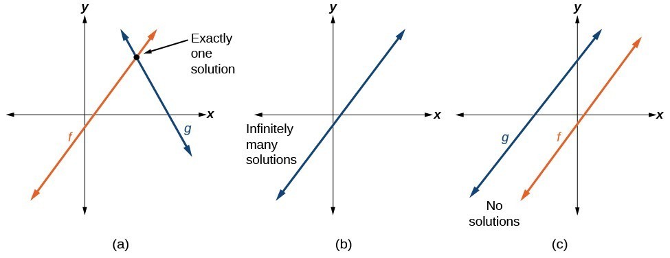
Real-world situations including two or more linear functions may be modeled with a system of linear equations . Remember, when solving a system of linear equations, we are looking for points the two lines have in common. Typically, there are three types of answers possible.
How To: Given a situation that represents a system of linear equations, write the system of equations and identify the solution.
- Identify the input and output of each linear model.
- Identify the slope and y -intercept of each linear model.
- Find the solution by setting the two linear functions equal to another and solving for x , or find the point of intersection on a graph.
Example 4: Building a System of Linear Models to Choose a Truck Rental Company
Jamal is choosing between two truck-rental companies. The first, Keep on Trucking, Inc., charges an up-front fee of $20, then 59 cents a mile. The second, Move It Your Way, charges an up-front fee of $16, then 63 cents a mile 1 . When will Keep on Trucking, Inc. be the better choice for Jamal?
The two important quantities in this problem are the cost and the number of miles driven. Because we have two companies to consider, we will define two functions.
| Input | , distance driven in miles |
| Outputs | ( ): cost, in dollars, for renting from Keep on Trucking ( ) cost, in dollars, for renting from Move It Your Way |
| Initial Value | Up-front fee: (0) = 20 and (0) = 16 |
| Rate of Change | ( ) = $0.59/mile and ( ) = $0.63/mile |
A linear function is of the form [latex]f\left(x\right)=mx+b[/latex]. Using the rates of change and initial charges, we can write the equations
[latex]\begin{gathered}K\left(d\right)=0.59d+20\\ M\left(d\right)=0.63d+16\end{gathered}[/latex]
Using these equations, we can determine when Keep on Trucking, Inc., will be the better choice. Because all we have to make that decision from is the costs, we are looking for when Move It Your Way, will cost less, or when [latex]K\left(d\right)<M\left(d\right)[/latex]. The solution pathway will lead us to find the equations for the two functions, find the intersection, and then see where the [latex]K\left(d\right)[/latex] function is smaller.
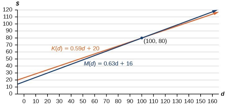
These graphs are sketched in Figure 7, with K ( d ) in blue.
To find the intersection, we set the equations equal and solve:
[latex]\begin{align}K\left(d\right)&=M\left(d\right) \\ 0.59d+20&=0.63d+16 \\ 4&=0.04d \\ 100&=d \\ d&=100 \end{align}[/latex]
This tells us that the cost from the two companies will be the same if 100 miles are driven. Either by looking at the graph, or noting that [latex]K\left(d\right)[/latex] is growing at a slower rate, we can conclude that Keep on Trucking, Inc. will be the cheaper price when more than 100 miles are driven, that is [latex]d>100[/latex].
- Precalculus. Authored by : OpenStax College. Provided by : OpenStax. Located at : http://cnx.org/contents/[email protected]:1/Preface . License : CC BY: Attribution
Linear Functions Problems with Solutions
Linear functions are highly used throughout mathematics and are therefore important to understand. A set of problems involving linear functions , along with detailed solutions, are presented. The problems are designed with emphasis on the meaning of the slope and the y intercept.
Problem 1: f is a linear function. Values of x and f(x) are given in the table below; complete the table.
Problem 2: A family of linear functions is given by
Solution to Problem 2: a)
Problem 3: A high school had 1200 students enrolled in 2003 and 1500 students in 2006. If the student population P ; grows as a linear function of time t, where t is the number of years after 2003. a) How many students will be enrolled in the school in 2010? b) Find a linear function that relates the student population to the time t. Solution to Problem 3: a) The given information may be written as ordered pairs (t , P). The year 2003 correspond to t = 0 and the year 2006 corresponds to t = 3, hence the 2 ordered pairs (0, 1200) and (3, 1500) Since the population grows linearly with the time t, we use the two ordered pairs to find the slope m of the graph of P as follows m = (1500 - 1200) / (6 - 3) = 100 students / year The slope m = 100 means that the students population grows by 100 students every year. From 2003 to 2010 there are 7 years and the students population in 2010 will be P(2010) = P(2003) + 7 * 100 = 1200 + 700 = 1900 students. b) We know the slope and two points, we may use the point slope form to find an equation for the population P as a function of t as follows P - P1 = m (t - t1) P - 1200 = 100 (t - 0) P = 100 t + 1200
Problem 4: The graph shown below is that of the linear function that relates the value V (in $) of a car to its age t, where t is the number of years after 2000.
Problem 5: The cost of producing x tools by a company is given by
Problem 6: A 500-liter tank full of oil is being drained at the constant rate of 20 liters par minute. a) Write a linear function V for the number of liters in the tank after t minutes (assuming that the drainage started at t = 0). b) Find the V and the t intercepts and interpret them. e) How many liters are in the tank after 11 minutes and 45 seconds? Solution to Problem 6: After each minute the amount of oil in the tank deceases by 20 liters. After t minutes, the amount of oil in the tank decreases by 20*t liters. Hence if at the start there 500 liters, after t minute the amount V of oil left in the tank is given by V = 500 - 20 t b) To find the V intercept, set t = 0 in the equation V = 500 - 20 t. V = 500 liters : it is the amount of oil at the start of the drainage. To find the t intercept, set V = 0 in the equation V = 500 - 20 t and solve for t. 0 = 500 - 20 t t = 500 / 20 = 25 minutes : it is the total time it takes to drain the 500 liters of oil. c) Convert 11 minutes 45 seconds in decimal form. t = 11 minutes 45 seconds = 11.75 minutes Calculate V at t = 11.75 minutes. V(11.75) = 500 - 20*11.75 = 265 liters are in the tank after 11 minutes 45 seconds of drainage.
Problem 7: A 50-meter by 70-meter rectangular garden is surrounded by a walkway of constant width x meters.
Problem 8: A driver starts a journey with 25 gallons in the tank of his car. The car burns 5 gallons for every 100 miles. Assuming that the amount of gasoline in the tank decreases linearly, a) write a linear function that relates the number of gallons G left in the tank after a journey of x miles. b) What is the value and meaning of the slope of the graph of G? c) What is the value and meaning of the x intercept? Solution to Problem 8: a) If 5 gallons are burnt for 100 miles then (5 / 100) gallons are burnt for 1 mile. Hence for x miles, x * (5 / 100) gallons are burnt. G is then equal to the initial amount of gasoline decreased by the amount gasoline burnt by the car. Hence G = 25 - (5 / 100) x b) The slope of G is equal to 5 / 1000 and it represent the amount of gasoline burnt for a distance of 1 mile. c) To find the x intercept, we set G = 0 and solve for x. 25 - (5 / 100) x = 0 x = 500 miles : it is the distance x for which all 25 gallons of gasoline will be burnt.
Problem 9: A rectangular wire frame has one of its dimensions moving at the rate of 0.5 cm / second. Its width is constant and equal to 4 cm. If at t = 0 the length of the rectangle is 10 cm,
2.3 Modeling with Linear Functions
Learning objectives.
In this section, you will:
- Identify steps for modeling and solving.
- Build linear models from verbal descriptions.
- Build systems of linear models.
Emily is a college student who plans to spend a summer in Seattle. She has saved $3,500 for her trip and anticipates spending $400 each week on rent, food, and activities. How can we write a linear model to represent her situation? What would be the x -intercept, and what can she learn from it? To answer these and related questions, we can create a model using a linear function. Models such as this one can be extremely useful for analyzing relationships and making predictions based on those relationships. In this section, we will explore examples of linear function models.
Identifying Steps to Model and Solve Problems
When modeling scenarios with linear functions and solving problems involving quantities with a constant rate of change , we typically follow the same problem strategies that we would use for any type of function. Let’s briefly review them:
- Identify changing quantities, and then define descriptive variables to represent those quantities. When appropriate, sketch a picture or define a coordinate system.
- Carefully read the problem to identify important information. Look for information that provides values for the variables or values for parts of the functional model, such as slope and initial value.
- Carefully read the problem to determine what we are trying to find, identify, solve, or interpret.
- Identify a solution pathway from the provided information to what we are trying to find. Often this will involve checking and tracking units, building a table, or even finding a formula for the function being used to model the problem.
- When needed, write a formula for the function.
- Solve or evaluate the function using the formula.
- Reflect on whether your answer is reasonable for the given situation and whether it makes sense mathematically.
- Clearly convey your result using appropriate units, and answer in full sentences when necessary.
Building Linear Models
Now let’s take a look at the student in Seattle. In her situation, there are two changing quantities: time and money. The amount of money she has remaining while on vacation depends on how long she stays. We can use this information to define our variables, including units.
- Output: M , M , money remaining, in dollars
- Input: t , t , time, in weeks
So, the amount of money remaining depends on the number of weeks: M ( t ) M ( t )
We can also identify the initial value and the rate of change.
- Initial Value: She saved $3,500, so $3,500 is the initial value for M . M .
- Rate of Change: She anticipates spending $400 each week, so –$400 per week is the rate of change, or slope.
Notice that the unit of dollars per week matches the unit of our output variable divided by our input variable. Also, because the slope is negative, the linear function is decreasing. This should make sense because she is spending money each week.
The rate of change is constant, so we can start with the linear model M ( t ) = m t + b . M ( t ) = m t + b . Then we can substitute the intercept and slope provided.
To find the x - x - intercept, we set the output to zero, and solve for the input.
The x - x - intercept is 8.75 weeks. Because this represents the input value when the output will be zero, we could say that Emily will have no money left after 8.75 weeks.
When modeling any real-life scenario with functions, there is typically a limited domain over which that model will be valid—almost no trend continues indefinitely. Here the domain refers to the number of weeks. In this case, it doesn’t make sense to talk about input values less than zero. A negative input value could refer to a number of weeks before she saved $3,500, but the scenario discussed poses the question once she saved $3,500 because this is when her trip and subsequent spending starts. It is also likely that this model is not valid after the x - x - intercept, unless Emily will use a credit card and goes into debt. The domain represents the set of input values, so the reasonable domain for this function is 0 ≤ t ≤ 8.75. 0 ≤ t ≤ 8.75.
In the above example, we were given a written description of the situation. We followed the steps of modeling a problem to analyze the information. However, the information provided may not always be the same. Sometimes we might be provided with an intercept. Other times we might be provided with an output value. We must be careful to analyze the information we are given, and use it appropriately to build a linear model.
Using a Given Intercept to Build a Model
Some real-world problems provide the y - y - intercept, which is the constant or initial value. Once the y - y - intercept is known, the x - x - intercept can be calculated. Suppose, for example, that Hannah plans to pay off a no-interest loan from her parents. Her loan balance is $1,000. She plans to pay $250 per month until her balance is $0. The y - y - intercept is the initial amount of her debt, or $1,000. The rate of change, or slope, is -$250 per month. We can then use the slope-intercept form and the given information to develop a linear model.
Now we can set the function equal to 0, and solve for x x to find the x - x - intercept.
The x - x - intercept is the number of months it takes her to reach a balance of $0. The x x -intercept is 4 months, so it will take Hannah four months to pay off her loan.
Using a Given Input and Output to Build a Model
Many real-world applications are not as direct as the ones we just considered. Instead they require us to identify some aspect of a linear function. We might sometimes instead be asked to evaluate the linear model at a given input or set the equation of the linear model equal to a specified output.
Given a word problem that includes two pairs of input and output values, use the linear function to solve a problem.
- Identify the input and output values.
- Convert the data to two coordinate pairs.
- Find the slope.
- Write the linear model.
- Use the model to make a prediction by evaluating the function at a given x - x - value.
- Use the model to identify an x - x - value that results in a given y - y - value.
- Answer the question posed.
Using a Linear Model to Investigate a Town’s Population
A town’s population has been growing linearly. In 2004 the population was 6,200. By 2009 the population had grown to 8,100. Assume this trend continues.
- ⓐ Predict the population in 2013.
- ⓑ Identify the year in which the population will reach 15,000.
The two changing quantities are the population size and time. While we could use the actual year value as the input quantity, doing so tends to lead to very cumbersome equations because the y - y - intercept would correspond to the year 0, more than 2000 years ago!
To make computation a little nicer, we will define our input as the number of years since 2004:
- Input: t , t , years since 2004
- Output: P ( t ) , P ( t ) , the town’s population
To predict the population in 2013 ( t = 9 ), ( t = 9 ), we would first need an equation for the population. Likewise, to find when the population would reach 15,000, we would need to solve for the input that would provide an output of 15,000. To write an equation, we need the initial value and the rate of change, or slope.
To determine the rate of change, we will use the change in output per change in input.
The problem gives us two input-output pairs. Converting them to match our defined variables, the year 2004 would correspond to t = 0 , t = 0 , giving the point ( 0 , 6200 ) . ( 0 , 6200 ) . Notice that through our clever choice of variable definition, we have “given” ourselves the y -intercept of the function. The year 2009 would correspond to t = 5, t = 5, giving the point ( 5 , 8100 ) . ( 5 , 8100 ) .
The two coordinate pairs are ( 0 , 6200 ) ( 0 , 6200 ) and ( 5 , 8100 ) . ( 5 , 8100 ) . Recall that we encountered examples in which we were provided two points earlier in the chapter. We can use these values to calculate the slope.
We already know the y -intercept of the line, so we can immediately write the equation:
To predict the population in 2013, we evaluate our function at t = 9. t = 9.
If the trend continues, our model predicts a population of 9,620 in 2013.
To find when the population will reach 15,000, we can set P ( t ) = 15000 P ( t ) = 15000 and solve for t . t .
Our model predicts the population will reach 15,000 in a little more than 23 years after 2004, or somewhere around the year 2027.
A company sells doughnuts. They incur a fixed cost of $25,000 for rent, insurance, and other expenses. It costs $0.25 to produce each doughnut.
- ⓐ Write a linear model to represent the cost C C of the company as a function of x , x , the number of doughnuts produced.
- ⓑ Find and interpret the y -intercept.
A city’s population has been growing linearly. In 2008, the population was 28,200. By 2012, the population was 36,800. Assume this trend continues.
- ⓐ Predict the population in 2014.
- ⓑ Identify the year in which the population will reach 54,000.
Using a Diagram to Model a Problem
It is useful for many real-world applications to draw a picture to gain a sense of how the variables representing the input and output may be used to answer a question. To draw the picture, first consider what the problem is asking for. Then, determine the input and the output. The diagram should relate the variables. Often, geometrical shapes or figures are drawn. Distances are often traced out. If a right triangle is sketched, the Pythagorean Theorem relates the sides. If a rectangle is sketched, labeling width and height is helpful.
Using a Diagram to Model Distance Walked
Anna and Emanuel start at the same intersection. Anna walks east at 4 miles per hour while Emanuel walks south at 3 miles per hour. They are communicating with a two-way radio that has a range of 2 miles. How long after they start walking will they fall out of radio contact?
In essence, we can partially answer this question by saying they will fall out of radio contact when they are 2 miles apart, which leads us to ask a new question:
“How long will it take them to be 2 miles apart?”
In this problem, our changing quantities are time and position, but ultimately we need to know how long will it take for them to be 2 miles apart. We can see that time will be our input variable, so we’ll define our input and output variables.
- Input: t , t , time in hours.
- Output: A ( t ) , A ( t ) , distance in miles, and E ( t ) , E ( t ) , distance in miles
Because it is not obvious how to define our output variable, we’ll start by drawing a picture such as Figure 2 .
Initial Value: They both start at the same intersection so when t = 0 , t = 0 , the distance traveled by each person should also be 0. Thus the initial value for each is 0.
Rate of Change: Anna is walking 4 miles per hour and Emanuel is walking 3 miles per hour, which are both rates of change. The slope for A A is 4 and the slope for E E is 3.
Using those values, we can write formulas for the distance each person has walked.
For this problem, the distances from the starting point are important. To notate these, we can define a coordinate system, identifying the “starting point” at the intersection where they both started. Then we can use the variable, A , A , which we introduced above, to represent Anna’s position, and define it to be a measurement from the starting point in the eastward direction. Likewise, can use the variable, E , E , to represent Emanuel’s position, measured from the starting point in the southward direction. Note that in defining the coordinate system, we specified both the starting point of the measurement and the direction of measure.
We can then define a third variable, D , D , to be the measurement of the distance between Anna and Emanuel. Showing the variables on the diagram is often helpful, as we can see from Figure 3 .
Recall that we need to know how long it takes for D , D , the distance between them, to equal 2 miles. Notice that for any given input t , t , the outputs A ( t ) , E ( t ) , A ( t ) , E ( t ) , and D ( t ) D ( t ) represent distances.
Figure 2 shows us that we can use the Pythagorean Theorem because we have drawn a right angle.
Using the Pythagorean Theorem, we get:
In this scenario we are considering only positive values of t , t , so our distance D ( t ) D ( t ) will always be positive. We can simplify this answer to D ( t ) = 5 t . D ( t ) = 5 t . This means that the distance between Anna and Emanuel is also a linear function. Because D D is a linear function, we can now answer the question of when the distance between them will reach 2 miles. We will set the output D ( t ) = 2 D ( t ) = 2 and solve for t . t .
They will fall out of radio contact in 0.4 hours, or 24 minutes.
Should I draw diagrams when given information based on a geometric shape?
Yes. Sketch the figure and label the quantities and unknowns on the sketch.
Using a Diagram to Model Distance between Cities
There is a straight road leading from the town of Westborough to Agritown 30 miles east and 10 miles north. Partway down this road, it junctions with a second road, perpendicular to the first, leading to the town of Eastborough. If the town of Eastborough is located 20 miles directly east of the town of Westborough, how far is the road junction from Westborough?
It might help here to draw a picture of the situation. See Figure 4 . It would then be helpful to introduce a coordinate system. While we could place the origin anywhere, placing it at Westborough seems convenient. This puts Agritown at coordinates ( 3 0 , 1 0 ) , ( 3 0 , 1 0 ) , and Eastborough at ( 2 0 , 0 ) . ( 2 0 , 0 ) .
Using this point along with the origin, we can find the slope of the line from Westborough to Agritown:
The equation of the road from Westborough to Agritown would be
From this, we can determine the perpendicular road to Eastborough will have slope m = – 3. m = – 3. Because the town of Eastborough is at the point (20, 0), we can find the equation:
We can now find the coordinates of the junction of the roads by finding the intersection of these lines. Setting them equal,
The roads intersect at the point (18, 6). Using the distance formula, we can now find the distance from Westborough to the junction.
One nice use of linear models is to take advantage of the fact that the graphs of these functions are lines. This means real-world applications discussing maps need linear functions to model the distances between reference points.
There is a straight road leading from the town of Timpson to Ashburn 60 miles east and 12 miles north. Partway down the road, it junctions with a second road, perpendicular to the first, leading to the town of Garrison. If the town of Garrison is located 22 miles directly east of the town of Timpson, how far is the road junction from Timpson?
Building Systems of Linear Models
Real-world situations including two or more linear functions may be modeled with a system of linear equations . Remember, when solving a system of linear equations, we are looking for points the two lines have in common. Typically, there are three types of answers possible, as shown in Figure 5 .
Given a situation that represents a system of linear equations, write the system of equations and identify the solution.
- Identify the input and output of each linear model.
- Identify the slope and y -intercept of each linear model.
- Find the solution by setting the two linear functions equal to one another and solving for x , x , or find the point of intersection on a graph.
Building a System of Linear Models to Choose a Truck Rental Company
Jamal is choosing between two truck-rental companies. The first, Keep on Trucking, Inc., charges an up-front fee of $20, then 59 cents a mile. The second, Move It Your Way, charges an up-front fee of $16, then 63 cents a mile 4 . When will Keep on Trucking, Inc. be the better choice for Jamal?
The two important quantities in this problem are the cost and the number of miles driven. Because we have two companies to consider, we will define two functions.
| Input | distance driven in miles |
| Outputs | cost, in dollars, for renting from Keep on Trucking cost, in dollars, for renting from Move It Your Way |
| Initial Value | Up-front fee: and |
| Rate of Change | /mile and /mile |
A linear function is of the form f ( x ) = m x + b . f ( x ) = m x + b . Using the rates of change and initial charges, we can write the equations
Using these equations, we can determine when Keep on Trucking, Inc., will be the better choice. Because all we have to make that decision from is the costs, we are looking for when Move It Your Way, will cost less, or when K ( d ) < M ( d ) . K ( d ) < M ( d ) . The solution pathway will lead us to find the equations for the two functions, find the intersection, and then see where the K ( d ) K ( d ) function is smaller.
These graphs are sketched in Figure 6 , with K ( d ) K ( d ) in blue.
To find the intersection, we set the equations equal and solve:
This tells us that the cost from the two companies will be the same if 100 miles are driven. Either by looking at the graph, or noting that K ( d ) K ( d ) is growing at a slower rate, we can conclude that Keep on Trucking, Inc. will be the cheaper price when more than 100 miles are driven, that is d > 100. d > 100.
Access this online resource for additional instruction and practice with linear function models.
- Interpreting a Linear Function
2.3 Section Exercises
Explain how to find the input variable in a word problem that uses a linear function.
Explain how to find the output variable in a word problem that uses a linear function.
Explain how to interpret the initial value in a word problem that uses a linear function.
Explain how to determine the slope in a word problem that uses a linear function.
Find the area of a parallelogram bounded by the y -axis, the line x = 3 , x = 3 , the line f ( x ) = 1 + 2 x , f ( x ) = 1 + 2 x , and the line parallel to f ( x ) f ( x ) passing through ( 2 , 7 ) . ( 2 , 7 ) .
Find the area of a triangle bounded by the x -axis, the line f ( x ) = 12 – 1 3 x , f ( x ) = 12 – 1 3 x , and the line perpendicular to f ( x ) f ( x ) that passes through the origin.
Find the area of a triangle bounded by the y -axis, the line f ( x ) = 9 – 6 7 x , f ( x ) = 9 – 6 7 x , and the line perpendicular to f ( x ) f ( x ) that passes through the origin.
Find the area of a parallelogram bounded by the x -axis, the line g ( x ) = 2 , g ( x ) = 2 , the line f ( x ) = 3 x , f ( x ) = 3 x , and the line parallel to f ( x ) f ( x ) passing through ( 6 , 1 ) . ( 6 , 1 ) .
For the following exercises, consider this scenario: A town’s population has been decreasing at a constant rate. In 2010 the population was 5,900. By 2012 the population had dropped 4,700. Assume this trend continues.
Predict the population in 2016.
Identify the year in which the population will reach 0.
For the following exercises, consider this scenario: A town’s population has been increased at a constant rate. In 2010 the population was 46,020. By 2012 the population had increased to 52,070. Assume this trend continues.
Identify the year in which the population will reach 75,000.
For the following exercises, consider this scenario: A town has an initial population of 75,000. It grows at a constant rate of 2,500 per year for 5 years.
Find the linear function that models the town’s population P P as a function of the year, t , t , where t t is the number of years since the model began.
Find a reasonable domain and range for the function P . P .
If the function P P is graphed, find and interpret the x - and y -intercepts.
If the function P P is graphed, find and interpret the slope of the function.
When will the output reached 100,000?
What is the output in the year 12 years from the onset of the model?
For the following exercises, consider this scenario: The weight of a newborn is 7.5 pounds. The baby gained one-half pound a month for its first year.
Find the linear function that models the baby’s weight W W as a function of the age of the baby, in months, t . t .
Find a reasonable domain and range for the function W W .
If the function W W is graphed, find and interpret the x - and y -intercepts.
If the function W is graphed, find and interpret the slope of the function.
When did the baby weight 10.4 pounds?
What is the output when the input is 6.2? Interpret your answer.
For the following exercises, consider this scenario: The number of people afflicted with the common cold in the winter months steadily decreased by 205 each year from 2005 until 2010. In 2005, 12,025 people were afflicted.
Find the linear function that models the number of people inflicted with the common cold C C as a function of the year, t . t .
Find a reasonable domain and range for the function C . C .
If the function C C is graphed, find and interpret the x - and y -intercepts.
If the function C C is graphed, find and interpret the slope of the function.
When will the output reach 0?
In what year will the number of people be 9,700?
For the following exercises, use the graph in Figure 7 , which shows the profit, y, y, in thousands of dollars, of a company in a given year, t, t, where t t represents the number of years since 1980.
Find the linear function y , y , where y y depends on t , t , the number of years since 1980.
Find and interpret the y -intercept.
Find and interpret the x -intercept.
Find and interpret the slope.
For the following exercises, use the graph in Figure 8 , which shows the profit, y , y , in thousands of dollars, of a company in a given year, t , t , where t t represents the number of years since 1980.
For the following exercises, use the median home values in Mississippi and Hawaii (adjusted for inflation) shown in Table 2 . Assume that the house values are changing linearly.
| Year | Mississippi | Hawaii |
|---|---|---|
| 1950 | $25,200 | $74,400 |
| 2000 | $71,400 | $272,700 |
In which state have home values increased at a higher rate?
If these trends were to continue, what would be the median home value in Mississippi in 2010?
If we assume the linear trend existed before 1950 and continues after 2000, the two states’ median house values will be (or were) equal in what year? (The answer might be absurd.)
For the following exercises, use the median home values in Indiana and Alabama (adjusted for inflation) shown in Table 3 . Assume that the house values are changing linearly.
| Year | Indiana | Alabama |
|---|---|---|
| 1950 | $37,700 | $27,100 |
| 2000 | $94,300 | $85,100 |
If these trends were to continue, what would be the median home value in Indiana in 2010?
Real-World Applications
In 2004, a school population was 1,001. By 2008 the population had grown to 1,697. Assume the population is changing linearly.
- ⓐ How much did the population grow between the year 2004 and 2008?
- ⓑ How long did it take the population to grow from 1,001 students to 1,697 students?
- ⓒ What is the average population growth per year?
- ⓓ What was the population in the year 2000?
- ⓔ Find an equation for the population, P , P , of the school t years after 2000.
- ⓕ Using your equation, predict the population of the school in 2011.
In 2003, a town’s population was 1,431. By 2007 the population had grown to 2,134. Assume the population is changing linearly.
- ⓐ How much did the population grow between the year 2003 and 2007?
- ⓑ How long did it take the population to grow from 1,431 people to 2,134 people?
- ⓔ Find an equation for the population, P P of the town t t years after 2000.
- ⓕ Using your equation, predict the population of the town in 2014.
A phone company has a monthly cellular plan where a customer pays a flat monthly fee and then a certain amount of money per minute used on the phone. If a customer uses 410 minutes, the monthly cost will be $71.50. If the customer uses 720 minutes, the monthly cost will be $118.
- ⓐ Find a linear equation for the monthly cost of the cell plan as a function of x , the number of monthly minutes used.
- ⓑ Interpret the slope and y -intercept of the equation.
- ⓒ Use your equation to find the total monthly cost if 687 minutes are used.
A phone company has a monthly cellular data plan where a customer pays a flat monthly fee of $10 and then a certain amount of money per megabyte (MB) of data used on the phone. If a customer uses 20 MB, the monthly cost will be $11.20. If the customer uses 130 MB, the monthly cost will be $17.80.
- ⓐ Find a linear equation for the monthly cost of the data plan as a function of x x , the number of MB used.
- ⓒ Use your equation to find the total monthly cost if 250 MB are used.
In 1991, the moose population in a park was measured to be 4,360. By 1999, the population was measured again to be 5,880. Assume the population continues to change linearly.
- ⓐ Find a formula for the moose population, P since 1990.
- ⓑ What does your model predict the moose population to be in 2003?
In 2003, the owl population in a park was measured to be 340. By 2007, the population was measured again to be 285. The population changes linearly. Let the input be years since 1990.
- ⓐ Find a formula for the owl population, P. P. Let the input be years since 2003.
- ⓑ What does your model predict the owl population to be in 2012?
The Federal Helium Reserve held about 16 billion cubic feet of helium in 2010 and is being depleted by about 2.1 billion cubic feet each year.
- ⓐ Give a linear equation for the remaining federal helium reserves, R, R, in terms of t, t, the number of years since 2010.
- ⓑ In 2015, what will the helium reserves be?
- ⓒ If the rate of depletion doesn’t change, in what year will the Federal Helium Reserve be depleted?
Suppose the world’s oil reserves in 2014 are 1,820 billion barrels. If, on average, the total reserves are decreasing by 25 billion barrels of oil each year:
- ⓐ Give a linear equation for the remaining oil reserves, R, R, in terms of t, t, the number of years since now.
- ⓑ Seven years from now, what will the oil reserves be?
- ⓒ If the rate at which the reserves are decreasing is constant, when will the world’s oil reserves be depleted?
You are choosing between two different prepaid cell phone plans. The first plan charges a rate of 26 cents per minute. The second plan charges a monthly fee of $19.95 plus 11 cents per minute. How many minutes would you have to use in a month in order for the second plan to be preferable?
You are choosing between two different window washing companies. The first charges $5 per window. The second charges a base fee of $40 plus $3 per window. How many windows would you need to have for the second company to be preferable?
When hired at a new job selling jewelry, you are given two pay options:
- Option A: Base salary of $17,000 a year with a commission of 12% of your sales
- Option B: Base salary of $20,000 a year with a commission of 5% of your sales
How much jewelry would you need to sell for option A to produce a larger income?
When hired at a new job selling electronics, you are given two pay options:
- Option A: Base salary of $14,000 a year with a commission of 10% of your sales
- Option B: Base salary of $19,000 a year with a commission of 4% of your sales
How much electronics would you need to sell for option A to produce a larger income?
- Option A: Base salary of $20,000 a year with a commission of 12% of your sales
- Option B: Base salary of $26,000 a year with a commission of 3% of your sales
- Option A: Base salary of $10,000 a year with a commission of 9% of your sales
- Option B: Base salary of $20,000 a year with a commission of 4% of your sales
- 4 Rates retrieved Aug 2, 2010 from http://www.budgettruck.com and http://www.uhaul.com/
This book may not be used in the training of large language models or otherwise be ingested into large language models or generative AI offerings without OpenStax's permission.
Want to cite, share, or modify this book? This book uses the Creative Commons Attribution License and you must attribute OpenStax.
Access for free at https://openstax.org/books/precalculus/pages/1-introduction-to-functions
- Authors: Jay Abramson
- Publisher/website: OpenStax
- Book title: Precalculus
- Publication date: Oct 23, 2014
- Location: Houston, Texas
- Book URL: https://openstax.org/books/precalculus/pages/1-introduction-to-functions
- Section URL: https://openstax.org/books/precalculus/pages/2-3-modeling-with-linear-functions
© Dec 8, 2021 OpenStax. Textbook content produced by OpenStax is licensed under a Creative Commons Attribution License . The OpenStax name, OpenStax logo, OpenStax book covers, OpenStax CNX name, and OpenStax CNX logo are not subject to the Creative Commons license and may not be reproduced without the prior and express written consent of Rice University.
A MIP-heuristic approach for solving a bi-objective optimization model for integrated production planning of sugarcane and energy-cane
- Original Research
- Published: 02 September 2024
Cite this article

- Gilmar Tolentino 1 na1 ,
- Antônio Roberto Balbo ORCID: orcid.org/0000-0002-4512-0140 1 na1 ,
- Sônia Cristina Poltroniere 1 na1 ,
- Angelo Aliano Filho ORCID: orcid.org/0000-0002-5088-134X 2 na1 &
- Helenice de Oliveira Florentino ORCID: orcid.org/0000-0003-2740-8826 3 na1
This paper proposes a modeling and solution approach for the integrated planning of the planting and harvesting of sucrose cane and energy-cane considering multiple harvesters. An integer linear bi-objective optimization model is proposed, which seeks to find a trade-off between the maximization of the production volumes of sucrose and fiber and the minimization of the operational costs. The model considers the technical constraints of the mill, such as the milling capacity and meeting the monthly demand. A MIP-heuristic based on relax-and-fix and fix-and-optimize strategies with exact decomposition is appropriately proposed to determine approximations to Pareto optimal solutions to this problem. These approximations are used as incumbents for a branch-and-bound tree to generate potentially Pareto optimal solutions. The results reveal that the MIP-heuristic efficiently solves the problem for real and semi-random instances, generating approximate solutions with a reduced error and a reasonable computational effort. Moreover, the different solutions quantify the trade-off between cost and production volume, opening up the possibility of increasing sucrose and fiber content or decreasing the costs of solutions found. Thus, the proposed bi-objective approach, the solution technique and the different Pareto optimal solutions obtained can assist mill managers in making better decisions in sugarcane production.
This is a preview of subscription content, log in via an institution to check access.
Access this article
Subscribe and save.
- Get 10 units per month
- Download Article/Chapter or eBook
- 1 Unit = 1 Article or 1 Chapter
- Cancel anytime
Price includes VAT (Russian Federation)
Instant access to the full article PDF.
Rent this article via DeepDyve
Institutional subscriptions

More details, see the Gurobi manual at https://www.gurobi.com/documentation/current/refman/heuristics.html.
Agarwal, A. K. (2007). Biofuels (alcohols and biodiesel) applications as fuels for internal combustion engines. Progress in Energy and Combustion Science, 33 (3), 233–271.
Article Google Scholar
Akartunali, K., & Miller, A. J. (2009). A heuristic approach for big bucket multi-level production planning problems. European Journal of Operational Research, 193 (2), 396–411. https://doi.org/10.1016/j.ejor.2007.11.033
Aliano, A. F., Cantane, D. R., Isler, P. R., & Florentino, H. O. (2023). An integrated multi-objective mathematical model for sugarcane harvesting considering cumulative degree-days. Expert Systems with Applications, 232 , 120881.
Aliano, A. F., Melo, T., & Pato, M. V. (2021). A bi-objective mathematical model for integrated planning of sugarcane harvesting and transport operations. Computers & Operations Research, 134 , 105419.
Aliano, A. F., Moretti, A. C., Pato, M. V., & de Oliveira, W. A. (2021). An exact scalarization method with multiple reference points for bi-objective integer linear optimization problems. Annals of Operations Research, 296 (1), 35–69.
Aliano, F. A., de Oliveira, W. A., & Melo, T. (2022). Multi-objective optimization for integrated sugarcane cultivation and harvesting planning. European Journal of Operational Research, 309 (1), 330–344.
Beraldi, P., Ghiani, G., Grieco, A., & Guerriero, E. (2008). Rolling-horizon and fix-and-relax heuristics for the parallel machine lot-sizing and scheduling problem with sequence-dependent set-up costs. Computers & Operations Research, 35 (11), 3644–3656.
Bezanson, J., Edelman, A., Karpinski, S., & Shah, V. B. (2017). Julia: A fresh approach to numerical computing. SIAM Review, 59 (1), 65–98.
Bigaton, A., Danelon, A. F., Bressan, G., Silva, H. J. T., & Rosa, J. H. M. (2017). Previsão de custos do setor sucroenergético na região centro-sul do Brasil: safra 2017/18. Revista IPecege, 3 (3), 65–70.
Bruzzone, A. A. G., Anghinolfi, D., Paolucci, M., & Tonelli, F. (2012). Energy-aware scheduling for improving manufacturing process sustainability: A mathematical model for flexible flow shops. CIRP Annals - Manufacturing Technology, 61 (1), 459–462.
Calija, V., Higgins, A. J., Jackson, P. A., Bielig, L. M., & Coomans, D. (2001). An operations research approach to the problem of the sugarcane selection. Annals of Operations Research, 108 (1–4), 123–142.
Cárdenas-Barrón, L. E., Melo, R. A., & Santos, M. C. (2021). Extended formulation and valid inequalities for the multi-item inventory lot-sizing problem with supplier selection. Computers and Operations Research, 130 , 105234.
Cheavegatti-Gianotto, A., de Abreu, H. M. C., Arruda, P., Bespalhok Filho, J. C., Burnquist, W. L., Creste, S., di Ciero, L., Ferro, J. A., et al. (2011). Sugarcane ( saccharum x officinarum ): A reference study for the regulation of genetically modified cultivars in brazil. Tropical Plant Biology, 4 , 62–89.
Chu, S., & Majumdar, A. (2012). Opportunities and challenges for a sustainable energy future. Nature, 488 (7411), 294–303.
Cunha, J. O., Mateus, G. R., & Melo, R. A. (2022). A hybrid heuristic for capacitated three-level lot-sizing and replenishment problems with a distribution structure. Computers and Industrial Engineering, 173 , 108698. https://doi.org/10.1016/j.cie.2022.108698
Danna, E., Rothberg, E., & Pape, C. L. (2005). Exploring relaxation induced neighborhoods to improve MIP solutions. Mathematical Programming, 102 , 71–90.
Dunning, I., Huchette, J., & Lubin, M. (2017). Jump: A modeling language for mathematical optimization. SIAM Review, 59 (2), 295–320.
Ehrgott, M., & Wiecek, M. M. (2005). Multiobjective programming. Multiple Criteria Decision Analysis: State of the Art Surveys, 78 , 667–708.
Google Scholar
Etemadnia, H., Goetz, S. J., Canning, P., & Tavallali, M. S. (2015). Optimal wholesale facilities location within the fruit and vegetables supply chain with bimodal transportation options: An lp-mip heuristic approach. European Journal of Operational Research, 244 (2), 648–661.
Farias, M. E. A., Martins, M. F., & Cândido, G. A. (2021). Agenda 2030 e energias renováveis: Sinergias e desafios para alcance do desenvolvimento sustentável. Research, Society and Development, 10 (17), e13101723867.
Ferreira, D., Morabito, R., & Rangel, S. (2009). Solution approaches for the soft drink integrated production lot sizing and scheduling problem. European Journal of Operational Research, 196 (2), 697–706. https://doi.org/10.1016/j.ejor.2008.03.035
Fischetti, M., & Lodi, A. (2003). Local branching. Mathematical Programming, 98 , 23–47.
Florentino, H. O., Irawan, C., Aliano, F. A., Jones, D. F., Cantane, D. R., & Nervis, J. J. (2018). A multiple objective methodology for sugarcane harvest management with varying maturation periods. Annals of Operations Research, 267 (1), 153–177.
Florentino, H. O., Jones, D. F., Irawan, C., Ouelhadj, D., Khosravi, B., & Cantane, D. R. (2020). An optimization model for combined selecting, planting and harvesting sugarcane varieties. Annals of Operations Research, 314 , 451–469.
Florentino, H. O., & Pato, M. V. (2014). A bi-objective genetic approach for the selection of sugarcane varieties to comply with environmental and economic requirements. Journal of the Operational Research Society, 65 (6), 842–854.
García-Segura, T., Penadés-Plà, V., & Yepes, V. (2018). Sustainable bridge design by metamodel-assisted multi-objective optimization and decision-making under uncertainty. Journal of Cleaner Production, 202 , 904–915.
Giagkiozis, I., & Fleming, P. J. (2015). Methods for multi-objective optimization: An analysis. Information Sciences, 293 , 338–350.
Gurobi Optimization, LLC: Gurobi Optimizer Reference Manual (2022). https://www.gurobi.com .
Helber, S., & Sahling, F. (2010). A fix-and-optimize approach for the multi-level capacitated lot sizing problem. International Journal of Production Economics, 123 (2), 247–256.
Higgins, A. (2006). Scheduling of road vehicles in sugarcane transport: A case study at an Australian sugar mill. European Journal of Operational Research, 170 (3), 987–1000.
Higgins, A., Antony, G., Sandell, G., Davies, I., Prestwidge, D., & Andrew, B. (2004). A framework for integrating a complex harvesting and transport system for sugar production. Agricultural Systems, 82 (2), 99–115.
Higgins, A. J., & Muchow, R. C. (2003). Assessing the potential benefits of alternative cane supply arrangements in the Australian sugar industry. Agricultural Systems, 76 (2), 623–638.
Higgins, A. J., & Postma, S. (2004). Australian sugar mills optimise siding rosters to increase profitability. Annals of Operations Research, 128 (1–4), 235–249.
James, R. J. W., & Almada-Lobo, B. (2011). Single and parallel machine capacitated lotsizing and scheduling: New iterative MIP-based neighborhood search heuristics. Computers and Operations Research, 38 (12), 1816–1825. https://doi.org/10.1016/j.cor.2011.02.005
Jena, S. D., & Poggi, M. (2013). Harvest planning in the Brazilian sugar cane industry via mixed integer programming. European Journal of Operational Research, 230 (2), 374–384.
Junqueira, R., & Morabito, R. (2019). Modeling and solving a sugarcane harvest front scheduling problem. International Journal of Production Economics, 213 , 150–160. https://doi.org/10.1016/j.ijpe.2019.03.009
Kaab, A., Sharifi, M., Mobli, H., Nabavi-Pelesaraei, A., & Chau, K. (2019). Use of optimization techniques for energy use efficiency and environmental life cycle assessment modification in sugarcane production. Energy, 181 , 1298–1320.
Kaewtrakulpong, K., Takigawa, T., Koike, M., Hasegawa, H., & Bahalayodhin, B. (2008). Truck allocation planning for cost reduction of mechanical sugarcane harvesting in Thailand an application of multi-objective optimization. Journal of the Japanese Society of Agricultural Machinery, 70 (2), 62–71.
Lamsal, K., Jones, P. C., & Thomas, B. W. (2017). Sugarcane harvest logistics in Brazil. Transportation Science, 51 (2), 771–789.
Liebman, M., & Dyck, E. (1993). Crop rotation and intercropping strategies for weed management. Ecological Applications, 3 (1), 92–122.
Lima, C., Balbo, A. R., Homem, T. P. D., & Florentino, H. O. (2017). A hybrid approach combining interior-point and branch-and-bound methods applied to the problem of sugar cane waste. Journal of the Operational Research Society, 68 (2), 147–164.
Matsuoka, S. & Rubio, L. C. S. (2019). Energy cane: A sound alternative of a bioenergy crop for tropics and subtropics. In Sugarcane Biofuels , pp. 39–66. Springer.
Matsuoka, S., dos Santos, E. G. D. & Tomazela, A. L. (2017). Free Fiber Level Drives Resilience and Hybrid Vigor in Energy Cane. LAP LAMBERT Academic Publishing.
Matsuoka, S., Rubio, L., Tomazela, A., & Santos, E. (2016). A evoluçao do proálcool. AgroANALYSIS, 36 (1), 29–30.
Miettinen, K. (1999). Nonlinear Multiobjective Optimization, vol. 12. Springer.
Milan, E. L., Fernandez, S. M., & Aragones, L. M. P. (2006). Sugar cane transportation in Cuba, a case study. European Journal of Operational Research, 174 (1), 374–386.
Muchow, R. C., Higgins, A. J., Rudd, A. V., & Ford, A. W. (1998). Optimising harvest date in sugar production: A case study for the Mossman mill region in Australia: II. sensitivity to crop age and crop class distribution. Field Crops Research, 57 (3), 243–251.
Nervis, J. J. (2015). Simulação para a otimização da colheita da cana-de-açúcar.
Nikulin, Y., Miettinen, K., & Mäkelä, M. M. (2012). A new achievement scalarizing function based on parameterization in multiobjective optimization. OR Spectrum, 34 (1), 69–87.
Pathumnakul, S., & Nakrachata-Amon, T. (2015). The applications of operations research in harvest planning: A case study of the sugarcane industry in Thailand. Journal of Japan Industrial Management Association, 65 (4E), 328–333.
Poltroniere, S. C., Aliano, F. A., Caversan, A. S., Balbo, A. R., & Florentino, H. O. (2021). Integrated planning for planting and harvesting sugarcane and energy-cane for the production of sucrose and energy. Computers and Electronics in Agriculture . https://doi.org/10.1016/j.compag.2020.105956
Pongpat, P., Mahmood, A., Ghani, H. U., Silalertruksa, T., & Gheewala, S. H. (2023). Optimization of food-fuel-fibre in biorefinery based on environmental and economic assessment: The case of sugarcane utilization in Thailand. Sustainable Production and Consumption, 37 , 398–411. https://doi.org/10.1016/j.spc.2023.03.013
Pornprakun, W., Sungnul, S., Kiataramkul, C., & Moore, E. J. (2019). Determining optimal policies for sugarcane harvesting in Thailand using bi-objective and quasi-newton optimization methods. Advances in Difference Equations, 2019 , 1–15.
Qiu, M., Meng, Y., Chen, J., Chen, Y., Li, Z., & Li, J. (2023). Dual multi-objective optimisation of the cane milling process. Computers & Industrial Engineering, 179 , 109146. https://doi.org/10.1016/j.cie.2023.109146
Ramos, R. P., Isler, P. R., Florentino, H. O., Jones, D., & Nervis, J. J. (2016). An optimization model for the combined planning and harvesting of sugarcane with maturity considerations. African Journal of Agricultural Research, 11 (40), 3950–3958.
Santoro, E., Soler, E. M., & Cherri, A. C. (2017). Route optimization in mechanized sugarcane harvesting. Computers and Electronics in Agriculture, 141 , 140–146.
Santos, J. A. (2022). Análise do sistema de energia fotovoltaica do Instituto Federal do Ceará-Campus Maracanaú e sua colaboração na redução da emissão de CO2. Available on: http://conexoes.ifce.edu.br/index.php/conexoes/article/view/2168 . Retrieved February 19, 2023.
Sethanan, K., & Neungmatcha, W. (2016). Multi-objective particle swarm optimization for mechanical harvester route planning of sugarcane field operations. European Journal of Operational Research, 252 (3), 969–984.
Shirvani, N., Ruiz, R., & Shadrokh, S. (2014). Cyclic scheduling of perishable products in parallel machine with release dates, due dates and deadlines. International Journal of Production Economics, 156 , 1–12.
Silva, A. F., Marins, F. A. S., & Dias, E. X. (2015). Addressing uncertainty in sugarcane harvest planning through a revised multi-choice goal programming model. Applied Mathematical Modelling, 39 (18), 5540–5558.
Toso, E. A., Morabito, R., & Clark, A. R. (2009). Lot sizing and sequencing optimisation at an animal-feed plant. Computers & Industrial Engineering, 57 (3), 813–821.
USDA: United States Department of Agriculture. (2023). Available on: https://apps.fas.usda.gov/psdonline/app/index.html#/app/advQuery . Retrieved January 31, 2023.
Usman, M., & Balsalobre-Lorente, D. (2022). Environmental concern in the era of industrialization: Can financial development, renewable energy and natural resources alleviate some load? Energy Policy, 162 , 112780.
Varshney, D., Mandade, P., & Shastri, Y. (2019). Multi-objective optimization of sugarcane bagasse utilization in an Indian sugar mill. Sustainable Production and Consumption, 18 , 96–114.
Walfrido, A. P., Luengo, C. A., Koehlinger, J., Garzone, P., & Cornacchia, G. (2008). Sugarcane energy use: The Cuban case. Energy policy, 36 (6), 2163–2181.
Download references
The authors thank to Brazilian foundations: CNPq n \(^{\textrm{o}}\) 306518/2022-8, CNPq n \(^{\textrm{o}}\) 304218/2022-7, FAPESP 2021/03039-1,FAPESP 2022/12652-1, PROPE/PROPG/UNESP/ FUNDUNESP grant 12/2022, for the financial support and language services provided.
Author information
Gilmar Tolentino, Antônio Roberto Balbo, Sônia Cristina Poltroniere, Angelo Aliano Filho and Helenice de Oliveira Florentino have contributed equally to this work.
Authors and Affiliations
Department of Mathematics, State University of Sao Paulo, Bauru, São Paulo, 17033-360, Brazil
Gilmar Tolentino, Antônio Roberto Balbo & Sônia Cristina Poltroniere
Department of Mathematics, Universidade Tecnológica Federal do Paraná, Apucarana, Paraná, 86812-460, Brazil
Angelo Aliano Filho
Department of Bioestatistics, State University of Sao Paulo, Botucatu, São Paulo, 18618-690, Brazil
Helenice de Oliveira Florentino
You can also search for this author in PubMed Google Scholar
Corresponding author
Correspondence to Angelo Aliano Filho .
Ethics declarations
Conflict of interest..
The authors declare to have no Conflict of interest.
Ethical approval.
This article does not contain any studies with human participants or animals performed by any of the authors.
Additional information
Publisher's note.
Springer Nature remains neutral with regard to jurisdictional claims in published maps and institutional affiliations.
Supplementary Information
Below is the link to the electronic supplementary material.
Supplementary file 1 (pdf 109 KB)
Rights and permissions.
Springer Nature or its licensor (e.g. a society or other partner) holds exclusive rights to this article under a publishing agreement with the author(s) or other rightsholder(s); author self-archiving of the accepted manuscript version of this article is solely governed by the terms of such publishing agreement and applicable law.
Reprints and permissions
About this article
Tolentino, G., Balbo, A.R., Poltroniere, S.C. et al. A MIP-heuristic approach for solving a bi-objective optimization model for integrated production planning of sugarcane and energy-cane. Ann Oper Res (2024). https://doi.org/10.1007/s10479-024-06229-5
Download citation
Received : 06 May 2023
Accepted : 16 August 2024
Published : 02 September 2024
DOI : https://doi.org/10.1007/s10479-024-06229-5
Share this article
Anyone you share the following link with will be able to read this content:
Sorry, a shareable link is not currently available for this article.
Provided by the Springer Nature SharedIt content-sharing initiative
- Multi-objective optimization
- Sugarcane production
- OR in agriculture
- MIP-heuristic
- Find a journal
- Publish with us
- Track your research
Information
- Author Services
Initiatives
You are accessing a machine-readable page. In order to be human-readable, please install an RSS reader.
All articles published by MDPI are made immediately available worldwide under an open access license. No special permission is required to reuse all or part of the article published by MDPI, including figures and tables. For articles published under an open access Creative Common CC BY license, any part of the article may be reused without permission provided that the original article is clearly cited. For more information, please refer to https://www.mdpi.com/openaccess .
Feature papers represent the most advanced research with significant potential for high impact in the field. A Feature Paper should be a substantial original Article that involves several techniques or approaches, provides an outlook for future research directions and describes possible research applications.
Feature papers are submitted upon individual invitation or recommendation by the scientific editors and must receive positive feedback from the reviewers.
Editor’s Choice articles are based on recommendations by the scientific editors of MDPI journals from around the world. Editors select a small number of articles recently published in the journal that they believe will be particularly interesting to readers, or important in the respective research area. The aim is to provide a snapshot of some of the most exciting work published in the various research areas of the journal.
Original Submission Date Received: .
- Active Journals
- Find a Journal
- Proceedings Series
- For Authors
- For Reviewers
- For Editors
- For Librarians
- For Publishers
- For Societies
- For Conference Organizers
- Open Access Policy
- Institutional Open Access Program
- Special Issues Guidelines
- Editorial Process
- Research and Publication Ethics
- Article Processing Charges
- Testimonials
- Preprints.org
- SciProfiles
- Encyclopedia
Article Menu

- Subscribe SciFeed
- Recommended Articles
- Google Scholar
- on Google Scholar
- Table of Contents
Find support for a specific problem in the support section of our website.
Please let us know what you think of our products and services.
Visit our dedicated information section to learn more about MDPI.
JSmol Viewer
Numerical algorithms for identification of convection coefficient and source in a magnetohydrodynamics flow.

1. Introduction
2. formulation of the direct and inverse problems, 2.1. the direct problem, 2.2. the inverse problems, 3. reduction of the ip1, ip2, and ip3 to nonclassical problems, 4. well-posedness of the inverse problems, 4.1. the ip2, 4.2. the ip1 and ip3, 5. finite difference approximation of the inverse problems, 6. algorithms for solution of finite difference algebraic systems, 6.1. the ip2, 6.2. the ip3 and ip1, 7. computational results, 7.1. inverse problem without noise, 7.2. inverse problem with a noise, 8. conclusions, author contributions, data availability statement, acknowledgments, conflicts of interest.
- Alifanov, O.M.; Artyukhin, E.A.; Rumyantsev, S.V. Extreme Methods for Solving Ill-Posed Problems with Applications to Inverse Heat Transfer Problems ; Begell House: New York, NY, USA; Wallingford, UK, 2015. [ Google Scholar ]
- Canon, J.R.; Van Der Hoek, J. Diffusion subject to the specification of mass. J. Math. Appl. 1986 , 115 , 517–529. [ Google Scholar ] [ CrossRef ]
- Kabanikhin, S.I. Inverse and Ill-Posed Problems Theory and Applications ; Walter de Gruyter: Berlin, Germany, 2011. [ Google Scholar ]
- Krukovskiy, A.J.; Poveschenko, J.A.; Podruga, V.O. Convergence of some iterative algorithms for numerical solution of two-dimentional non-stationary problems of magnetic hydrodynamics. Math. Model. 2023 , 35 , 57–74. (In Russian) [ Google Scholar ]
- Ladyzhenskaia, V.A.; Solonnikov, V.A.; Ural’tceva, N.N. Linear and Quasi-linear Equations of Parabolic Type ; American Mathematical Society: Providence, RI, USA, 1986. [ Google Scholar ]
- Samarskii, A.A.; Vabishchevich, P.N. Numerical Methods for Solving Inverse Problems of Mathematical Physics ; Walter de Gruyter: Berlin, Germany, 2007. [ Google Scholar ]
- Vabishchevich, P.N.; Vasil’ev, V.I. Computational determination of the lowest order coefficient in a parabolic equation. Dokl. Math. 2014 , 89 , 179–181. [ Google Scholar ] [ CrossRef ]
- Vabishchevich, P.N.; Vasil’ev, V.I. Computational algorithms for solving the coefficient inverse problem for parabolic equations. Inv. Probl. Sci. Eng. 2016 , 24 , 42–59. [ Google Scholar ] [ CrossRef ]
- Ashyraliev, A.; Sazaklioglu, A.V. Investgation of a time-dependent source identification with integral overdetermination. Numer. Funct. Anal. Optim. 2017 , 38 , 1276–1294. [ Google Scholar ] [ CrossRef ]
- Borzi, A. Modelling with Ordinary Differential Equations. A Comprehensive Approach ; Chapman and Hall, CRC Press: Boca Raton, FL, USA, 2020. [ Google Scholar ]
- Georgiev, S.G.; Vulkov, L.V. Computational recovery of time-dependent volatility from integral observations in option pricing. J. Comput. Sci. 2019 , 39 , 101054. [ Google Scholar ] [ CrossRef ]
- Glotov, D.; Hames, W.E.; Meir, A.J.; Ngoma, S. An integral constrained parabolic problem with applications in thermochronology. Comput. Math. Appl. 2016 , 71 , 2301–2312. [ Google Scholar ] [ CrossRef ]
- Glotov, D.; Hames, W.E.; Meir, A.J.; Ngoma, S. An inverse diffusion coefficient problem for a parabolic equation with integral constraint. Int. J. Numer. Anal. Model. 2018 , 15 , 552–563. [ Google Scholar ]
- Evans, L.C. Partial Differential Equations , 2nd ed.; Graduate Studies in Mathematics 19; American Mathematical Society: Providence, RI, USA, 2010. [ Google Scholar ]
- He, Y. Unconditional convergence of the Euler semi-implicit scheme for the three dimensional incompressible MHD equations. IMA J. Numer. Anal. 2015 , 33 , 767–801. [ Google Scholar ] [ CrossRef ]
- Isakov, V. Inverse Problems for Partial Differential Equations , 2nd ed.; Springer: New York, NY, USA, 2006. [ Google Scholar ]
- Landau, L.D.; Bell, J.; Kearsley, M.; Pitaevski, L.; Lifshitz, E.; Sykes, J. Electrodynamics of Continuous Media ; Elsevier: Amsterdam, The Netherlands, 2013; eBook ISBN 9781483293752. [ Google Scholar ]
- Nguyen, T.N.O. Source identification for parabolic equations from integral observations by the finite difference splitting method. Acta Math. Vietnam. 2024 , 49 , 283–308. [ Google Scholar ]
- Samarskii, A.A.; Nikolaev, E.S. Numerical Methods for Grid Equations: Volume I Direct Methods ; Birkhäuser Verlag: Berlin, Germany, 1989. [ Google Scholar ]
- Slodicka, M.; Seliga, L. Identification of memory kernels in hyperbolic problems. J. Comp. Appl. Math. 2017 , 311 , 618–629. [ Google Scholar ] [ CrossRef ]
- Tsyba, V.; Chebatorev, A.Y. Optimal control asymptotics of a magnetohydrodynamic flow. Comp. Math. Math. Phys. 2009 , 49 , 466–473. [ Google Scholar ] [ CrossRef ]
- Marchuk, G.I. Adjoint Equations and Analysis of Complex Systems ; Kluwer Acad. Publishers: Dordrecht, The Netherlands, 1995. [ Google Scholar ]
- Koleva, M.N.; Vulkov, L.G. A Galerkin finite element method for reconstruction of time-dependent convection coefficients and source in a 1-D model of magnetohydrodynamics. Appl. Sci. 2024 , 14 , 5949. [ Google Scholar ] [ CrossRef ]
- Ren, Z.; Guo, S.; Li, Z.; Wu, Z. Adjoint-based parameter and state estimation in 1-D magnetohydrodynamics (MHD) flow system. J. Optim. Manag. Optim. 2018 , 14 , 1579–1594. [ Google Scholar ] [ CrossRef ]
- Yu, P.X.; Tian, Z.F. Comparison of the simplified and full MHD models for laminar incompressible flow past a circular cylinder. Appl. Math. Model. 2017 , 41 , 143–163. [ Google Scholar ] [ CrossRef ]
- Khankishiyev, Z.F. Solution of one problem for linear loaded parabolic type differential equation with integral conditions. Adv. Math. Mod. Appl. 2022 , 7 , 178–190. [ Google Scholar ]
- Vabishchevich, P.N.; Klibanov, M.V. Numerical identification of the leading coefficient of a parabolic equation. Differ. Equ. 2016 , 52 , 855–862. [ Google Scholar ] [ CrossRef ]
- Kandilarov, J.; Vulkov, L. Simultaneous numerical reconstruction of time-dependent convection coefficient and source in magnetohydrodynamics flow system. In Proceedings of the 16th Annual Meeting of the Bulgarian Section of SIAM, (BGSIAM’21) (to Appear), Sofia, Bulgaria, 21–23 December 2021. [ Google Scholar ]
Click here to enlarge figure
| u | B | f | ||||||||
|---|---|---|---|---|---|---|---|---|---|---|
| Ratio | Order | Ratio | Order | Ratio | Order | |||||
| 5 | 5 | 9.2310e-03 | - | - | 6.5473e-04 | - | - | 1.1485e-02 | ||
| 10 | 10 | 5.0943e-03 | 1.81 | 0.86 | 1.6591e-04 | 3.95 | 1.98 | 6.1159e-03 | 1.88 | 0.91 |
| 20 | 20 | 2.6823e-03 | 1.90 | 0.93 | 4.5833e-05 | 3.60 | 1.85 | 3.1974e-03 | 1.91 | 0.94 |
| 40 | 40 | 1.3803e-03 | 1.94 | 0.96 | 1.6712e-05 | 2.72 | 1.45 | 1.6416e-03 | 1.95 | 0.96 |
| 80 | 80 | 7.0073e-04 | 1.97 | 0.98 | 7.1775e-06 | 2.32 | 1.21 | 8.3274e-04 | 1.97 | 0.98 |
| 160 | 160 | 3.5312e-04 | 1.98 | 0.99 | 3.3274e-06 | 2.14 | 1.11 | 4.1952e-04 | 1.99 | 0.99 |
| ffl | 0 | 0.0005 | 0.001 | 0.01 | 0.1 |
|---|---|---|---|---|---|
| u | 1.3803e-03 | 1.3638e-03 | 1.5238e-03 | 2.1379e-03 | 1.6747e-02 |
| B | 1.6712e-05 | 1.6546e-05 | 1.6297e-05 | 2.5556e-05 | 1.6864e-04 |
| f | 1.6416e-03 | 1.8412e-03 | 1.9766e-03 | 7.8766e-03 | 6.8009e-02 |
| The statements, opinions and data contained in all publications are solely those of the individual author(s) and contributor(s) and not of MDPI and/or the editor(s). MDPI and/or the editor(s) disclaim responsibility for any injury to people or property resulting from any ideas, methods, instructions or products referred to in the content. |
Share and Cite
Kandilarov, J.D.; Vulkov, L.G. Numerical Algorithms for Identification of Convection Coefficient and Source in a Magnetohydrodynamics Flow. Algorithms 2024 , 17 , 387. https://doi.org/10.3390/a17090387
Kandilarov JD, Vulkov LG. Numerical Algorithms for Identification of Convection Coefficient and Source in a Magnetohydrodynamics Flow. Algorithms . 2024; 17(9):387. https://doi.org/10.3390/a17090387
Kandilarov, Juri D., and Lubin G. Vulkov. 2024. "Numerical Algorithms for Identification of Convection Coefficient and Source in a Magnetohydrodynamics Flow" Algorithms 17, no. 9: 387. https://doi.org/10.3390/a17090387
Article Metrics
Article access statistics, further information, mdpi initiatives, follow mdpi.
Subscribe to receive issue release notifications and newsletters from MDPI journals
IMAGES
VIDEO
COMMENTS
Identifying Steps to Model and Solve Problems. When modeling scenarios with linear functions and solving problems involving quantities with a constant rate of change, we typically follow the same problem strategies that we would use for any type of function.Let's briefly review them: Identify changing quantities, and then define descriptive variables to represent those quantities.
When building linear models to solve problems involving quantities with a constant rate of change, we typically follow the same problem strategies that we would use for any type of function. Let's briefly review them: Identify changing quantities, and then define descriptive variables to represent those quantities. When appropriate, sketch a ...
Applying Linear Models. Modeling linear relationships can help solve real-world applications. Consider the example situations below, and note how different problem-solving methods may be used in each. Nadia has $200 in her savings account. She gets a job that pays $7.50 per hour and she deposits all her earnings in her savings account.
The rate of change is constant, so we can start with the linear model M (t)= mt+b M (t) = m t + b. Then we can substitute the intercept and slope provided. To find the x -intercept, we set the output to zero and solve for the input. 0= −400t+3500 t= 3500 400 t= 8.75 0 = − 400 t + 3500 t = 3500 400 t = 8.75. The x -intercept is 8.75 weeks.
How To: Given a word problem that includes two pairs of input and output values, use the linear function to solve a problem. Identify the input and output values. Convert the data to two coordinate pairs. Find the slope. Write the linear model. Use the model to make a prediction by evaluating the function at a given x value.
When modeling scenarios with a linear function and solving problems involving quantities changing linearly, ... Find a linear model for the value, then find and interpret the horizontal intercept and determine a reasonable domain and range for this function. Solution. In the problem, there are two changing quantities: time and value. The ...
Setting Up a Linear Equation to Solve a Real-World Application. There are two cell phone companies that offer different packages. Company A charges a monthly service fee of $34 plus $.05/min talk-time. Company B charges a monthly service fee of $40 plus $.04/min talk-time. ⓐ Write a linear equation that models the packages offered by both ...
Any situation that has a "constant rate of change" is a linear model. There are many common examples of linear models, including sales tax, linear depreciation, hourly salary, and the grade (steepness) of a road. In Preparation M.2, various definitions for linear models were presented. In this collaboration, we will use these definitions ...
A linear model is usually described by two parameters: the slope, often called the growth factor or rate of change, and the y y -intercept, often called the initial value. Given the slope m m and the y y -intercept b, b, the linear model can be written as a linear function y = mx + b. y = mx+b. We can represent the position of a car moving at a ...
Courses on Khan Academy are always 100% free. Start practicing—and saving your progress—now: https://www.khanacademy.org/math/algebra-home/alg-linear-eq-fun...
A linear programming problem with a bounded set always has an optimal solution. This means that a bounded set has a maximum value as well as a minimum value. Example 1: Given the objective function P = 10 x − 3 y and the following feasible set, Find the maximum value and the point where the maximum occurs.
If there are two decision variables in a linear programming problem then the graphical method can be used to solve such a problem easily. Suppose we have to maximize Z = 2x + 5y. The constraints are x + 4y ≤ 24, 3x + y ≤ 21 and x + y ≤ 9. where, x ≥ 0 and y ≥ 0. To solve this problem using the graphical method the steps are as follows.
Explanation: For example making a graph of temperature vs volume can be used to predict a value for absolute zero. The linear line can be extended to find a predicted value for the temperature where there is zero volume. The place on the line where volume is zero would be predict value for absolute zero. David Drayer · 1 · Aug 6 2018.
The process of minimizing a linear objective function subject to a finite number of linear equality and inequality constraints. The word "programming" is historical and predates computer programming. Quintessential tool for optimal allocation of scarce resources, among a number of competing activities.
Use this model to predict how much the car will be worth in 2020. Solution: We let \(x\) = the number of years after 2010, and let \(y\) = the cost. Solving this problem is equivalent to finding an equation of a line that passes through the points (0, 16800) and (4, 12000). To find the linear model for this problem, we need to find the slope.
Show Details. Learn how to solve real-world problems using linear modeling. MAT.ALG.409.0501 (Applications of Linear Interpolation and Extrapolation - Algebra)
If this problem persists, tell us. Our mission is to provide a free, world-class education to anyone, anywhere. Khan Academy is a 501(c)(3) nonprofit organization. Donate or volunteer today! Site Navigation. About. News; Impact; Our team; Our interns; Our content specialists; Our leadership; Our supporters; Our contributors; Our finances;
2. Fitting a Linear Model. In order to fit linear regression models in R, lm can be used for linear models, which are specified symbolically. A typical model takes the form of response~predictors where response is the (numeric) response vector and predictors is a series of predictor variables.
How To: Given a word problem that includes two pairs of input and output values, use the linear function to solve a problem. Identify the input and output values. Convert the data to two coordinate pairs. Find the slope. Write the linear model. Use the model to make a prediction by evaluating the function at a given x value.
The problems are designed with emphasis on the meaning of the slope and the y intercept. Problem 1: f is a linear function. Values of x and f(x) are given in the table below; complete the table. Solution to Problem 1: f is a linear function whose formula has the form f(x) = a x + b where a and b are constants to be found. Note that 2 ordered ...
Exercise 2.7.1.2. Find a linear equation to model this real-world application: It costs ABC electronics company $2.50 per unit to produce a part used in a popular brand of desktop computers. The company has monthly operating expenses of $350 for utilities and $3, 300 for salaries.
Given a word problem that includes two pairs of input and output values, use the linear function to solve a problem. Identify the input and output values. Convert the data to two coordinate pairs. Find the slope. Write the linear model. Use the model to make a prediction by evaluating the function at a given x-x-value.
This paper proposes a modeling and solution approach for the integrated planning of the planting and harvesting of sucrose cane and energy-cane considering multiple harvesters. An integer linear bi-objective optimization model is proposed, which seeks to find a trade-off between the maximization of the production volumes of sucrose and fiber and the minimization of the operational costs. The ...
We consider three integral observations inverse problems (IP1, IP2, IP3) for reconstruction of a time-dependent convection coefficient and a source in magnetohydrodynamics (MHD) model. On the first stage, using the integral observations, we reduce the inverse problems to nonclassical direct (forward) ones. The equivalence between the inverse and direct problems is established. Then, the well ...