hypothesis testing as maths questions

AS Level Mechanics and Statistics - Hypothesis Testing

Hypothesis Testing

This page looks at Hypothesis testing. Topics include null hypothesis, alternative hypothesis, testing and critical regions.

The parameters of a distribution are those quantities that you need to specify when describing the distribution. For example, a normal distribution has parameters μ and σ 2 and a Poisson distribution has parameter λ.

If we know that some data comes from a certain distribution, but the parameter is unknown, we might try to predict what the parameter is. Hypothesis testing is about working out how likely our predictions are.

The null hypothesis , denoted by H 0 , is a prediction about a parameter (so if we are dealing with a normal distribution, we might predict the mean or the variance of the distribution).

We also have an alternative hypothesis , denoted by H 1 . We then perform a test to decide whether or not we should reject the null hypothesis in favour of the alternative.

Suppose we are given a value and told that it comes from a certain distribution, but we don"t know what the parameter of that distribution is.

Suppose we make a null hypothesis about the parameter. We test how likely it is that the value we were given could have come from the distribution with this predicted parameter.

For example, suppose we are told that the value of 3 has come from a Poisson distribution. We might want to test the null hypothesis that the parameter (which is the mean) of the Poisson distribution is 9. So we work out how likely it is that the value of 3 could have come from a Poisson distribution with parameter 9. If it"s not very likely, we reject the null hypothesis in favour of the alternative.

Critical Region

But what exactly is "not very likely"?

We choose a region known as the critical region . If the result of our test lies in this region, then we reject the null hypothesis in favour of the alternative.

• school Campus Bookshelves
• menu_book Bookshelves
• perm_media Learning Objects
• login Login
• how_to_reg Request Instructor Account
• hub Instructor Commons

Margin Size

• Download Page (PDF)
• Download Full Book (PDF)
• Periodic Table
• Physics Constants
• Scientific Calculator
• Reference & Cite
• Tools expand_more
• Readability

selected template will load here

This action is not available.

9.1: Introduction to Hypothesis Testing

• Last updated
• Save as PDF
• Page ID 10211

• Kyle Siegrist
• University of Alabama in Huntsville via Random Services

\( \newcommand{\vecs}[1]{\overset { \scriptstyle \rightharpoonup} {\mathbf{#1}} } \)

\( \newcommand{\vecd}[1]{\overset{-\!-\!\rightharpoonup}{\vphantom{a}\smash {#1}}} \)

\( \newcommand{\id}{\mathrm{id}}\) \( \newcommand{\Span}{\mathrm{span}}\)

( \newcommand{\kernel}{\mathrm{null}\,}\) \( \newcommand{\range}{\mathrm{range}\,}\)

\( \newcommand{\RealPart}{\mathrm{Re}}\) \( \newcommand{\ImaginaryPart}{\mathrm{Im}}\)

\( \newcommand{\Argument}{\mathrm{Arg}}\) \( \newcommand{\norm}[1]{\| #1 \|}\)

\( \newcommand{\inner}[2]{\langle #1, #2 \rangle}\)

\( \newcommand{\Span}{\mathrm{span}}\)

\( \newcommand{\id}{\mathrm{id}}\)

\( \newcommand{\kernel}{\mathrm{null}\,}\)

\( \newcommand{\range}{\mathrm{range}\,}\)

\( \newcommand{\RealPart}{\mathrm{Re}}\)

\( \newcommand{\ImaginaryPart}{\mathrm{Im}}\)

\( \newcommand{\Argument}{\mathrm{Arg}}\)

\( \newcommand{\norm}[1]{\| #1 \|}\)

\( \newcommand{\Span}{\mathrm{span}}\) \( \newcommand{\AA}{\unicode[.8,0]{x212B}}\)

\( \newcommand{\vectorA}[1]{\vec{#1}}      % arrow\)

\( \newcommand{\vectorAt}[1]{\vec{\text{#1}}}      % arrow\)

\( \newcommand{\vectorB}[1]{\overset { \scriptstyle \rightharpoonup} {\mathbf{#1}} } \)

\( \newcommand{\vectorC}[1]{\textbf{#1}} \)

\( \newcommand{\vectorD}[1]{\overrightarrow{#1}} \)

\( \newcommand{\vectorDt}[1]{\overrightarrow{\text{#1}}} \)

\( \newcommand{\vectE}[1]{\overset{-\!-\!\rightharpoonup}{\vphantom{a}\smash{\mathbf {#1}}}} \)

Basic Theory

Preliminaries.

As usual, our starting point is a random experiment with an underlying sample space and a probability measure \(\P\). In the basic statistical model, we have an observable random variable \(\bs{X}\) taking values in a set \(S\). In general, \(\bs{X}\) can have quite a complicated structure. For example, if the experiment is to sample \(n\) objects from a population and record various measurements of interest, then \[ \bs{X} = (X_1, X_2, \ldots, X_n) \] where \(X_i\) is the vector of measurements for the \(i\)th object. The most important special case occurs when \((X_1, X_2, \ldots, X_n)\) are independent and identically distributed. In this case, we have a random sample of size \(n\) from the common distribution.

The purpose of this section is to define and discuss the basic concepts of statistical hypothesis testing . Collectively, these concepts are sometimes referred to as the Neyman-Pearson framework, in honor of Jerzy Neyman and Egon Pearson, who first formalized them.

A statistical hypothesis is a statement about the distribution of \(\bs{X}\). Equivalently, a statistical hypothesis specifies a set of possible distributions of \(\bs{X}\): the set of distributions for which the statement is true. A hypothesis that specifies a single distribution for \(\bs{X}\) is called simple ; a hypothesis that specifies more than one distribution for \(\bs{X}\) is called composite .

In hypothesis testing , the goal is to see if there is sufficient statistical evidence to reject a presumed null hypothesis in favor of a conjectured alternative hypothesis . The null hypothesis is usually denoted \(H_0\) while the alternative hypothesis is usually denoted \(H_1\).

An hypothesis test is a statistical decision ; the conclusion will either be to reject the null hypothesis in favor of the alternative, or to fail to reject the null hypothesis. The decision that we make must, of course, be based on the observed value \(\bs{x}\) of the data vector \(\bs{X}\). Thus, we will find an appropriate subset \(R\) of the sample space \(S\) and reject \(H_0\) if and only if \(\bs{x} \in R\). The set \(R\) is known as the rejection region or the critical region . Note the asymmetry between the null and alternative hypotheses. This asymmetry is due to the fact that we assume the null hypothesis, in a sense, and then see if there is sufficient evidence in \(\bs{x}\) to overturn this assumption in favor of the alternative.

An hypothesis test is a statistical analogy to proof by contradiction, in a sense. Suppose for a moment that \(H_1\) is a statement in a mathematical theory and that \(H_0\) is its negation. One way that we can prove \(H_1\) is to assume \(H_0\) and work our way logically to a contradiction. In an hypothesis test, we don't prove anything of course, but there are similarities. We assume \(H_0\) and then see if the data \(\bs{x}\) are sufficiently at odds with that assumption that we feel justified in rejecting \(H_0\) in favor of \(H_1\).

Often, the critical region is defined in terms of a statistic \(w(\bs{X})\), known as a test statistic , where \(w\) is a function from \(S\) into another set \(T\). We find an appropriate rejection region \(R_T \subseteq T\) and reject \(H_0\) when the observed value \(w(\bs{x}) \in R_T\). Thus, the rejection region in \(S\) is then \(R = w^{-1}(R_T) = \left\{\bs{x} \in S: w(\bs{x}) \in R_T\right\}\). As usual, the use of a statistic often allows significant data reduction when the dimension of the test statistic is much smaller than the dimension of the data vector.

The ultimate decision may be correct or may be in error. There are two types of errors, depending on which of the hypotheses is actually true.

Types of errors:

• A type 1 error is rejecting the null hypothesis \(H_0\) when \(H_0\) is true.
• A type 2 error is failing to reject the null hypothesis \(H_0\) when the alternative hypothesis \(H_1\) is true.

Similarly, there are two ways to make a correct decision: we could reject \(H_0\) when \(H_1\) is true or we could fail to reject \(H_0\) when \(H_0\) is true. The possibilities are summarized in the following table:

Of course, when we observe \(\bs{X} = \bs{x}\) and make our decision, either we will have made the correct decision or we will have committed an error, and usually we will never know which of these events has occurred. Prior to gathering the data, however, we can consider the probabilities of the various errors.

If \(H_0\) is true (that is, the distribution of \(\bs{X}\) is specified by \(H_0\)), then \(\P(\bs{X} \in R)\) is the probability of a type 1 error for this distribution. If \(H_0\) is composite, then \(H_0\) specifies a variety of different distributions for \(\bs{X}\) and thus there is a set of type 1 error probabilities.

The maximum probability of a type 1 error, over the set of distributions specified by \( H_0 \), is the significance level of the test or the size of the critical region.

The significance level is often denoted by \(\alpha\). Usually, the rejection region is constructed so that the significance level is a prescribed, small value (typically 0.1, 0.05, 0.01).

If \(H_1\) is true (that is, the distribution of \(\bs{X}\) is specified by \(H_1\)), then \(\P(\bs{X} \notin R)\) is the probability of a type 2 error for this distribution. Again, if \(H_1\) is composite then \(H_1\) specifies a variety of different distributions for \(\bs{X}\), and thus there will be a set of type 2 error probabilities. Generally, there is a tradeoff between the type 1 and type 2 error probabilities. If we reduce the probability of a type 1 error, by making the rejection region \(R\) smaller, we necessarily increase the probability of a type 2 error because the complementary region \(S \setminus R\) is larger.

The extreme cases can give us some insight. First consider the decision rule in which we never reject \(H_0\), regardless of the evidence \(\bs{x}\). This corresponds to the rejection region \(R = \emptyset\). A type 1 error is impossible, so the significance level is 0. On the other hand, the probability of a type 2 error is 1 for any distribution defined by \(H_1\). At the other extreme, consider the decision rule in which we always rejects \(H_0\) regardless of the evidence \(\bs{x}\). This corresponds to the rejection region \(R = S\). A type 2 error is impossible, but now the probability of a type 1 error is 1 for any distribution defined by \(H_0\). In between these two worthless tests are meaningful tests that take the evidence \(\bs{x}\) into account.

If \(H_1\) is true, so that the distribution of \(\bs{X}\) is specified by \(H_1\), then \(\P(\bs{X} \in R)\), the probability of rejecting \(H_0\) is the power of the test for that distribution.

Thus the power of the test for a distribution specified by \( H_1 \) is the probability of making the correct decision.

Suppose that we have two tests, corresponding to rejection regions \(R_1\) and \(R_2\), respectively, each having significance level \(\alpha\). The test with region \(R_1\) is uniformly more powerful than the test with region \(R_2\) if \[ \P(\bs{X} \in R_1) \ge \P(\bs{X} \in R_2) \text{ for every distribution of } \bs{X} \text{ specified by } H_1 \]

Naturally, in this case, we would prefer the first test. Often, however, two tests will not be uniformly ordered; one test will be more powerful for some distributions specified by \(H_1\) while the other test will be more powerful for other distributions specified by \(H_1\).

If a test has significance level \(\alpha\) and is uniformly more powerful than any other test with significance level \(\alpha\), then the test is said to be a uniformly most powerful test at level \(\alpha\).

Clearly a uniformly most powerful test is the best we can do.

\(P\)-value

In most cases, we have a general procedure that allows us to construct a test (that is, a rejection region \(R_\alpha\)) for any given significance level \(\alpha \in (0, 1)\). Typically, \(R_\alpha\) decreases (in the subset sense) as \(\alpha\) decreases.

The \(P\)-value of the observed value \(\bs{x}\) of \(\bs{X}\), denoted \(P(\bs{x})\), is defined to be the smallest \(\alpha\) for which \(\bs{x} \in R_\alpha\); that is, the smallest significance level for which \(H_0\) is rejected, given \(\bs{X} = \bs{x}\).

Knowing \(P(\bs{x})\) allows us to test \(H_0\) at any significance level for the given data \(\bs{x}\): If \(P(\bs{x}) \le \alpha\) then we would reject \(H_0\) at significance level \(\alpha\); if \(P(\bs{x}) \gt \alpha\) then we fail to reject \(H_0\) at significance level \(\alpha\). Note that \(P(\bs{X})\) is a statistic . Informally, \(P(\bs{x})\) can often be thought of as the probability of an outcome as or more extreme than the observed value \(\bs{x}\), where extreme is interpreted relative to the null hypothesis \(H_0\).

Analogy with Justice Systems

There is a helpful analogy between statistical hypothesis testing and the criminal justice system in the US and various other countries. Consider a person charged with a crime. The presumed null hypothesis is that the person is innocent of the crime; the conjectured alternative hypothesis is that the person is guilty of the crime. The test of the hypotheses is a trial with evidence presented by both sides playing the role of the data. After considering the evidence, the jury delivers the decision as either not guilty or guilty . Note that innocent is not a possible verdict of the jury, because it is not the point of the trial to prove the person innocent. Rather, the point of the trial is to see whether there is sufficient evidence to overturn the null hypothesis that the person is innocent in favor of the alternative hypothesis of that the person is guilty. A type 1 error is convicting a person who is innocent; a type 2 error is acquitting a person who is guilty. Generally, a type 1 error is considered the more serious of the two possible errors, so in an attempt to hold the chance of a type 1 error to a very low level, the standard for conviction in serious criminal cases is beyond a reasonable doubt .

Tests of an Unknown Parameter

Hypothesis testing is a very general concept, but an important special class occurs when the distribution of the data variable \(\bs{X}\) depends on a parameter \(\theta\) taking values in a parameter space \(\Theta\). The parameter may be vector-valued, so that \(\bs{\theta} = (\theta_1, \theta_2, \ldots, \theta_n)\) and \(\Theta \subseteq \R^k\) for some \(k \in \N_+\). The hypotheses generally take the form \[ H_0: \theta \in \Theta_0 \text{ versus } H_1: \theta \notin \Theta_0 \] where \(\Theta_0\) is a prescribed subset of the parameter space \(\Theta\). In this setting, the probabilities of making an error or a correct decision depend on the true value of \(\theta\). If \(R\) is the rejection region, then the power function \( Q \) is given by \[ Q(\theta) = \P_\theta(\bs{X} \in R), \quad \theta \in \Theta \] The power function gives a lot of information about the test.

The power function satisfies the following properties:

• \(Q(\theta)\) is the probability of a type 1 error when \(\theta \in \Theta_0\).
• \(\max\left\{Q(\theta): \theta \in \Theta_0\right\}\) is the significance level of the test.
• \(1 - Q(\theta)\) is the probability of a type 2 error when \(\theta \notin \Theta_0\).
• \(Q(\theta)\) is the power of the test when \(\theta \notin \Theta_0\).

If we have two tests, we can compare them by means of their power functions.

Suppose that we have two tests, corresponding to rejection regions \(R_1\) and \(R_2\), respectively, each having significance level \(\alpha\). The test with rejection region \(R_1\) is uniformly more powerful than the test with rejection region \(R_2\) if \( Q_1(\theta) \ge Q_2(\theta)\) for all \( \theta \notin \Theta_0 \).

Most hypothesis tests of an unknown real parameter \(\theta\) fall into three special cases:

Suppose that \( \theta \) is a real parameter and \( \theta_0 \in \Theta \) a specified value. The tests below are respectively the two-sided test , the left-tailed test , and the right-tailed test .

• \(H_0: \theta = \theta_0\) versus \(H_1: \theta \ne \theta_0\)
• \(H_0: \theta \ge \theta_0\) versus \(H_1: \theta \lt \theta_0\)
• \(H_0: \theta \le \theta_0\) versus \(H_1: \theta \gt \theta_0\)

Thus the tests are named after the conjectured alternative. Of course, there may be other unknown parameters besides \(\theta\) (known as nuisance parameters ).

Equivalence Between Hypothesis Test and Confidence Sets

There is an equivalence between hypothesis tests and confidence sets for a parameter \(\theta\).

Suppose that \(C(\bs{x})\) is a \(1 - \alpha\) level confidence set for \(\theta\). The following test has significance level \(\alpha\) for the hypothesis \( H_0: \theta = \theta_0 \) versus \( H_1: \theta \ne \theta_0 \): Reject \(H_0\) if and only if \(\theta_0 \notin C(\bs{x})\)

By definition, \(\P[\theta \in C(\bs{X})] = 1 - \alpha\). Hence if \(H_0\) is true so that \(\theta = \theta_0\), then the probability of a type 1 error is \(P[\theta \notin C(\bs{X})] = \alpha\).

Equivalently, we fail to reject \(H_0\) at significance level \(\alpha\) if and only if \(\theta_0\) is in the corresponding \(1 - \alpha\) level confidence set. In particular, this equivalence applies to interval estimates of a real parameter \(\theta\) and the common tests for \(\theta\) given above .

In each case below, the confidence interval has confidence level \(1 - \alpha\) and the test has significance level \(\alpha\).

• Suppose that \(\left[L(\bs{X}, U(\bs{X})\right]\) is a two-sided confidence interval for \(\theta\). Reject \(H_0: \theta = \theta_0\) versus \(H_1: \theta \ne \theta_0\) if and only if \(\theta_0 \lt L(\bs{X})\) or \(\theta_0 \gt U(\bs{X})\).
• Suppose that \(L(\bs{X})\) is a confidence lower bound for \(\theta\). Reject \(H_0: \theta \le \theta_0\) versus \(H_1: \theta \gt \theta_0\) if and only if \(\theta_0 \lt L(\bs{X})\).
• Suppose that \(U(\bs{X})\) is a confidence upper bound for \(\theta\). Reject \(H_0: \theta \ge \theta_0\) versus \(H_1: \theta \lt \theta_0\) if and only if \(\theta_0 \gt U(\bs{X})\).

Pivot Variables and Test Statistics

Recall that confidence sets of an unknown parameter \(\theta\) are often constructed through a pivot variable , that is, a random variable \(W(\bs{X}, \theta)\) that depends on the data vector \(\bs{X}\) and the parameter \(\theta\), but whose distribution does not depend on \(\theta\) and is known. In this case, a natural test statistic for the basic tests given above is \(W(\bs{X}, \theta_0)\).

Reset password New user? Sign up

Existing user? Log in

Hypothesis Testing

Already have an account? Log in here.

A hypothesis test is a statistical inference method used to test the significance of a proposed (hypothesized) relation between population statistics (parameters) and their corresponding sample estimators . In other words, hypothesis tests are used to determine if there is enough evidence in a sample to prove a hypothesis true for the entire population.

The test considers two hypotheses: the null hypothesis , which is a statement meant to be tested, usually something like "there is no effect" with the intention of proving this false, and the alternate hypothesis , which is the statement meant to stand after the test is performed. The two hypotheses must be mutually exclusive ; moreover, in most applications, the two are complementary (one being the negation of the other). The test works by comparing the \(p\)-value to the level of significance (a chosen target). If the \(p\)-value is less than or equal to the level of significance, then the null hypothesis is rejected.

When analyzing data, only samples of a certain size might be manageable as efficient computations. In some situations the error terms follow a continuous or infinite distribution, hence the use of samples to suggest accuracy of the chosen test statistics. The method of hypothesis testing gives an advantage over guessing what distribution or which parameters the data follows.

Definitions and Methodology

Hypothesis test and confidence intervals.

In statistical inference, properties (parameters) of a population are analyzed by sampling data sets. Given assumptions on the distribution, i.e. a statistical model of the data, certain hypotheses can be deduced from the known behavior of the model. These hypotheses must be tested against sampled data from the population.

The null hypothesis \((\)denoted \(H_0)\) is a statement that is assumed to be true. If the null hypothesis is rejected, then there is enough evidence (statistical significance) to accept the alternate hypothesis \((\)denoted \(H_1).\) Before doing any test for significance, both hypotheses must be clearly stated and non-conflictive, i.e. mutually exclusive, statements. Rejecting the null hypothesis, given that it is true, is called a type I error and it is denoted \(\alpha\), which is also its probability of occurrence. Failing to reject the null hypothesis, given that it is false, is called a type II error and it is denoted \(\beta\), which is also its probability of occurrence. Also, \(\alpha\) is known as the significance level , and \(1-\beta\) is known as the power of the test. \(H_0\) \(\textbf{is true}\)\(\hspace{15mm}\) \(H_0\) \(\textbf{is false}\) \(\textbf{Reject}\) \(H_0\)\(\hspace{10mm}\) Type I error Correct Decision \(\textbf{Reject}\) \(H_1\) Correct Decision Type II error The test statistic is the standardized value following the sampled data under the assumption that the null hypothesis is true, and a chosen particular test. These tests depend on the statistic to be studied and the assumed distribution it follows, e.g. the population mean following a normal distribution. The \(p\)-value is the probability of observing an extreme test statistic in the direction of the alternate hypothesis, given that the null hypothesis is true. The critical value is the value of the assumed distribution of the test statistic such that the probability of making a type I error is small.

Methodologies: Given an estimator \(\hat \theta\) of a population statistic \(\theta\), following a probability distribution \(P(T)\), computed from a sample \(\mathcal{S},\) and given a significance level \(\alpha\) and test statistic \(t^*,\) define \(H_0\) and \(H_1;\) compute the test statistic \(t^*.\) \(p\)-value Approach (most prevalent): Find the \(p\)-value using \(t^*\) (right-tailed). If the \(p\)-value is at most \(\alpha,\) reject \(H_0\). Otherwise, reject \(H_1\). Critical Value Approach: Find the critical value solving the equation \(P(T\geq t_\alpha)=\alpha\) (right-tailed). If \(t^*>t_\alpha\), reject \(H_0\). Otherwise, reject \(H_1\). Note: Failing to reject \(H_0\) only means inability to accept \(H_1\), and it does not mean to accept \(H_0\).

Assume a normally distributed population has recorded cholesterol levels with various statistics computed. From a sample of 100 subjects in the population, the sample mean was 214.12 mg/dL (milligrams per deciliter), with a sample standard deviation of 45.71 mg/dL. Perform a hypothesis test, with significance level 0.05, to test if there is enough evidence to conclude that the population mean is larger than 200 mg/dL. Hypothesis Test We will perform a hypothesis test using the \(p\)-value approach with significance level \(\alpha=0.05:\) Define \(H_0\): \(\mu=200\). Define \(H_1\): \(\mu>200\). Since our values are normally distributed, the test statistic is \(z^*=\frac{\bar X - \mu_0}{\frac{s}{\sqrt{n}}}=\frac{214.12 - 200}{\frac{45.71}{\sqrt{100}}}\approx 3.09\). Using a standard normal distribution, we find that our \(p\)-value is approximately \(0.001\). Since the \(p\)-value is at most \(\alpha=0.05,\) we reject \(H_0\). Therefore, we can conclude that the test shows sufficient evidence to support the claim that \(\mu\) is larger than \(200\) mg/dL.

If the sample size was smaller, the normal and \(t\)-distributions behave differently. Also, the question itself must be managed by a double-tail test instead.

Assume a population's cholesterol levels are recorded and various statistics are computed. From a sample of 25 subjects, the sample mean was 214.12 mg/dL (milligrams per deciliter), with a sample standard deviation of 45.71 mg/dL. Perform a hypothesis test, with significance level 0.05, to test if there is enough evidence to conclude that the population mean is not equal to 200 mg/dL. Hypothesis Test We will perform a hypothesis test using the \(p\)-value approach with significance level \(\alpha=0.05\) and the \(t\)-distribution with 24 degrees of freedom: Define \(H_0\): \(\mu=200\). Define \(H_1\): \(\mu\neq 200\). Using the \(t\)-distribution, the test statistic is \(t^*=\frac{\bar X - \mu_0}{\frac{s}{\sqrt{n}}}=\frac{214.12 - 200}{\frac{45.71}{\sqrt{25}}}\approx 1.54\). Using a \(t\)-distribution with 24 degrees of freedom, we find that our \(p\)-value is approximately \(2(0.068)=0.136\). We have multiplied by two since this is a two-tailed argument, i.e. the mean can be smaller than or larger than. Since the \(p\)-value is larger than \(\alpha=0.05,\) we fail to reject \(H_0\). Therefore, the test does not show sufficient evidence to support the claim that \(\mu\) is not equal to \(200\) mg/dL.

The complement of the rejection on a two-tailed hypothesis test (with significance level \(\alpha\)) for a population parameter \(\theta\) is equivalent to finding a confidence interval \((\)with confidence level \(1-\alpha)\) for the population parameter \(\theta\). If the assumption on the parameter \(\theta\) falls inside the confidence interval, then the test has failed to reject the null hypothesis \((\)with \(p\)-value greater than \(\alpha).\) Otherwise, if \(\theta\) does not fall in the confidence interval, then the null hypothesis is rejected in favor of the alternate \((\)with \(p\)-value at most \(\alpha).\)

• Statistics (Estimation)
• Normal Distribution
• Correlation
• Confidence Intervals

Problem Loading...

Note Loading...

Set Loading...

If you're seeing this message, it means we're having trouble loading external resources on our website.

If you're behind a web filter, please make sure that the domains *.kastatic.org and *.kasandbox.org are unblocked.

To log in and use all the features of Khan Academy, please enable JavaScript in your browser.

Statistics and probability

Course: statistics and probability   >   unit 12, hypothesis testing and p-values.

• One-tailed and two-tailed tests
• Z-statistics vs. T-statistics
• Small sample hypothesis test
• Large sample proportion hypothesis testing

Want to join the conversation?

• Upvote Button navigates to signup page
• Downvote Button navigates to signup page
• Flag Button navigates to signup page

Video transcript

Hypothesis Testing

Hypothesis testing is a tool for making statistical inferences about the population data. It is an analysis tool that tests assumptions and determines how likely something is within a given standard of accuracy. Hypothesis testing provides a way to verify whether the results of an experiment are valid.

A null hypothesis and an alternative hypothesis are set up before performing the hypothesis testing. This helps to arrive at a conclusion regarding the sample obtained from the population. In this article, we will learn more about hypothesis testing, its types, steps to perform the testing, and associated examples.

What is Hypothesis Testing in Statistics?

Hypothesis testing uses sample data from the population to draw useful conclusions regarding the population probability distribution . It tests an assumption made about the data using different types of hypothesis testing methodologies. The hypothesis testing results in either rejecting or not rejecting the null hypothesis.

Hypothesis Testing Definition

Hypothesis testing can be defined as a statistical tool that is used to identify if the results of an experiment are meaningful or not. It involves setting up a null hypothesis and an alternative hypothesis. These two hypotheses will always be mutually exclusive. This means that if the null hypothesis is true then the alternative hypothesis is false and vice versa. An example of hypothesis testing is setting up a test to check if a new medicine works on a disease in a more efficient manner.

Null Hypothesis

The null hypothesis is a concise mathematical statement that is used to indicate that there is no difference between two possibilities. In other words, there is no difference between certain characteristics of data. This hypothesis assumes that the outcomes of an experiment are based on chance alone. It is denoted as \(H_{0}\). Hypothesis testing is used to conclude if the null hypothesis can be rejected or not. Suppose an experiment is conducted to check if girls are shorter than boys at the age of 5. The null hypothesis will say that they are the same height.

Alternative Hypothesis

The alternative hypothesis is an alternative to the null hypothesis. It is used to show that the observations of an experiment are due to some real effect. It indicates that there is a statistical significance between two possible outcomes and can be denoted as \(H_{1}\) or \(H_{a}\). For the above-mentioned example, the alternative hypothesis would be that girls are shorter than boys at the age of 5.

Hypothesis Testing P Value

In hypothesis testing, the p value is used to indicate whether the results obtained after conducting a test are statistically significant or not. It also indicates the probability of making an error in rejecting or not rejecting the null hypothesis.This value is always a number between 0 and 1. The p value is compared to an alpha level, \(\alpha\) or significance level. The alpha level can be defined as the acceptable risk of incorrectly rejecting the null hypothesis. The alpha level is usually chosen between 1% to 5%.

Hypothesis Testing Critical region

All sets of values that lead to rejecting the null hypothesis lie in the critical region. Furthermore, the value that separates the critical region from the non-critical region is known as the critical value.

Hypothesis Testing Formula

Depending upon the type of data available and the size, different types of hypothesis testing are used to determine whether the null hypothesis can be rejected or not. The hypothesis testing formula for some important test statistics are given below:

• z = \(\frac{\overline{x}-\mu}{\frac{\sigma}{\sqrt{n}}}\). \(\overline{x}\) is the sample mean, \(\mu\) is the population mean, \(\sigma\) is the population standard deviation and n is the size of the sample.
• t = \(\frac{\overline{x}-\mu}{\frac{s}{\sqrt{n}}}\). s is the sample standard deviation.
• \(\chi ^{2} = \sum \frac{(O_{i}-E_{i})^{2}}{E_{i}}\). \(O_{i}\) is the observed value and \(E_{i}\) is the expected value.

We will learn more about these test statistics in the upcoming section.

Types of Hypothesis Testing

Selecting the correct test for performing hypothesis testing can be confusing. These tests are used to determine a test statistic on the basis of which the null hypothesis can either be rejected or not rejected. Some of the important tests used for hypothesis testing are given below.

Hypothesis Testing Z Test

A z test is a way of hypothesis testing that is used for a large sample size (n ≥ 30). It is used to determine whether there is a difference between the population mean and the sample mean when the population standard deviation is known. It can also be used to compare the mean of two samples. It is used to compute the z test statistic. The formulas are given as follows:

• One sample: z = \(\frac{\overline{x}-\mu}{\frac{\sigma}{\sqrt{n}}}\).
• Two samples: z = \(\frac{(\overline{x_{1}}-\overline{x_{2}})-(\mu_{1}-\mu_{2})}{\sqrt{\frac{\sigma_{1}^{2}}{n_{1}}+\frac{\sigma_{2}^{2}}{n_{2}}}}\).

Hypothesis Testing t Test

The t test is another method of hypothesis testing that is used for a small sample size (n < 30). It is also used to compare the sample mean and population mean. However, the population standard deviation is not known. Instead, the sample standard deviation is known. The mean of two samples can also be compared using the t test.

• One sample: t = \(\frac{\overline{x}-\mu}{\frac{s}{\sqrt{n}}}\).
• Two samples: t = \(\frac{(\overline{x_{1}}-\overline{x_{2}})-(\mu_{1}-\mu_{2})}{\sqrt{\frac{s_{1}^{2}}{n_{1}}+\frac{s_{2}^{2}}{n_{2}}}}\).

Hypothesis Testing Chi Square

The Chi square test is a hypothesis testing method that is used to check whether the variables in a population are independent or not. It is used when the test statistic is chi-squared distributed.

One Tailed Hypothesis Testing

One tailed hypothesis testing is done when the rejection region is only in one direction. It can also be known as directional hypothesis testing because the effects can be tested in one direction only. This type of testing is further classified into the right tailed test and left tailed test.

Right Tailed Hypothesis Testing

The right tail test is also known as the upper tail test. This test is used to check whether the population parameter is greater than some value. The null and alternative hypotheses for this test are given as follows:

\(H_{0}\): The population parameter is ≤ some value

\(H_{1}\): The population parameter is > some value.

If the test statistic has a greater value than the critical value then the null hypothesis is rejected

Left Tailed Hypothesis Testing

The left tail test is also known as the lower tail test. It is used to check whether the population parameter is less than some value. The hypotheses for this hypothesis testing can be written as follows:

\(H_{0}\): The population parameter is ≥ some value

\(H_{1}\): The population parameter is < some value.

The null hypothesis is rejected if the test statistic has a value lesser than the critical value.

Two Tailed Hypothesis Testing

In this hypothesis testing method, the critical region lies on both sides of the sampling distribution. It is also known as a non - directional hypothesis testing method. The two-tailed test is used when it needs to be determined if the population parameter is assumed to be different than some value. The hypotheses can be set up as follows:

\(H_{0}\): the population parameter = some value

\(H_{1}\): the population parameter ≠ some value

The null hypothesis is rejected if the test statistic has a value that is not equal to the critical value.

Hypothesis Testing Steps

Hypothesis testing can be easily performed in five simple steps. The most important step is to correctly set up the hypotheses and identify the right method for hypothesis testing. The basic steps to perform hypothesis testing are as follows:

• Step 1: Set up the null hypothesis by correctly identifying whether it is the left-tailed, right-tailed, or two-tailed hypothesis testing.
• Step 2: Set up the alternative hypothesis.
• Step 3: Choose the correct significance level, \(\alpha\), and find the critical value.
• Step 4: Calculate the correct test statistic (z, t or \(\chi\)) and p-value.
• Step 5: Compare the test statistic with the critical value or compare the p-value with \(\alpha\) to arrive at a conclusion. In other words, decide if the null hypothesis is to be rejected or not.

Hypothesis Testing Example

The best way to solve a problem on hypothesis testing is by applying the 5 steps mentioned in the previous section. Suppose a researcher claims that the mean average weight of men is greater than 100kgs with a standard deviation of 15kgs. 30 men are chosen with an average weight of 112.5 Kgs. Using hypothesis testing, check if there is enough evidence to support the researcher's claim. The confidence interval is given as 95%.

Step 1: This is an example of a right-tailed test. Set up the null hypothesis as \(H_{0}\): \(\mu\) = 100.

Step 2: The alternative hypothesis is given by \(H_{1}\): \(\mu\) > 100.

Step 3: As this is a one-tailed test, \(\alpha\) = 100% - 95% = 5%. This can be used to determine the critical value.

1 - \(\alpha\) = 1 - 0.05 = 0.95

0.95 gives the required area under the curve. Now using a normal distribution table, the area 0.95 is at z = 1.645. A similar process can be followed for a t-test. The only additional requirement is to calculate the degrees of freedom given by n - 1.

Step 4: Calculate the z test statistic. This is because the sample size is 30. Furthermore, the sample and population means are known along with the standard deviation.

z = \(\frac{\overline{x}-\mu}{\frac{\sigma}{\sqrt{n}}}\).

\(\mu\) = 100, \(\overline{x}\) = 112.5, n = 30, \(\sigma\) = 15

z = \(\frac{112.5-100}{\frac{15}{\sqrt{30}}}\) = 4.56

Step 5: Conclusion. As 4.56 > 1.645 thus, the null hypothesis can be rejected.

Hypothesis Testing and Confidence Intervals

Confidence intervals form an important part of hypothesis testing. This is because the alpha level can be determined from a given confidence interval. Suppose a confidence interval is given as 95%. Subtract the confidence interval from 100%. This gives 100 - 95 = 5% or 0.05. This is the alpha value of a one-tailed hypothesis testing. To obtain the alpha value for a two-tailed hypothesis testing, divide this value by 2. This gives 0.05 / 2 = 0.025.

Related Articles:

• Probability and Statistics
• Data Handling

Important Notes on Hypothesis Testing

• Hypothesis testing is a technique that is used to verify whether the results of an experiment are statistically significant.
• It involves the setting up of a null hypothesis and an alternate hypothesis.
• There are three types of tests that can be conducted under hypothesis testing - z test, t test, and chi square test.
• Hypothesis testing can be classified as right tail, left tail, and two tail tests.

Examples on Hypothesis Testing

• Example 1: The average weight of a dumbbell in a gym is 90lbs. However, a physical trainer believes that the average weight might be higher. A random sample of 5 dumbbells with an average weight of 110lbs and a standard deviation of 18lbs. Using hypothesis testing check if the physical trainer's claim can be supported for a 95% confidence level. Solution: As the sample size is lesser than 30, the t-test is used. \(H_{0}\): \(\mu\) = 90, \(H_{1}\): \(\mu\) > 90 \(\overline{x}\) = 110, \(\mu\) = 90, n = 5, s = 18. \(\alpha\) = 0.05 Using the t-distribution table, the critical value is 2.132 t = \(\frac{\overline{x}-\mu}{\frac{s}{\sqrt{n}}}\) t = 2.484 As 2.484 > 2.132, the null hypothesis is rejected. Answer: The average weight of the dumbbells may be greater than 90lbs
• Example 2: The average score on a test is 80 with a standard deviation of 10. With a new teaching curriculum introduced it is believed that this score will change. On random testing, the score of 38 students, the mean was found to be 88. With a 0.05 significance level, is there any evidence to support this claim? Solution: This is an example of two-tail hypothesis testing. The z test will be used. \(H_{0}\): \(\mu\) = 80, \(H_{1}\): \(\mu\) ≠ 80 \(\overline{x}\) = 88, \(\mu\) = 80, n = 36, \(\sigma\) = 10. \(\alpha\) = 0.05 / 2 = 0.025 The critical value using the normal distribution table is 1.96 z = \(\frac{\overline{x}-\mu}{\frac{\sigma}{\sqrt{n}}}\) z = \(\frac{88-80}{\frac{10}{\sqrt{36}}}\) = 4.8 As 4.8 > 1.96, the null hypothesis is rejected. Answer: There is a difference in the scores after the new curriculum was introduced.
• Example 3: The average score of a class is 90. However, a teacher believes that the average score might be lower. The scores of 6 students were randomly measured. The mean was 82 with a standard deviation of 18. With a 0.05 significance level use hypothesis testing to check if this claim is true. Solution: The t test will be used. \(H_{0}\): \(\mu\) = 90, \(H_{1}\): \(\mu\) < 90 \(\overline{x}\) = 110, \(\mu\) = 90, n = 6, s = 18 The critical value from the t table is -2.015 t = \(\frac{\overline{x}-\mu}{\frac{s}{\sqrt{n}}}\) t = \(\frac{82-90}{\frac{18}{\sqrt{6}}}\) t = -1.088 As -1.088 > -2.015, we fail to reject the null hypothesis. Answer: There is not enough evidence to support the claim.

go to slide go to slide go to slide

Book a Free Trial Class

FAQs on Hypothesis Testing

What is hypothesis testing.

Hypothesis testing in statistics is a tool that is used to make inferences about the population data. It is also used to check if the results of an experiment are valid.

What is the z Test in Hypothesis Testing?

The z test in hypothesis testing is used to find the z test statistic for normally distributed data . The z test is used when the standard deviation of the population is known and the sample size is greater than or equal to 30.

What is the t Test in Hypothesis Testing?

The t test in hypothesis testing is used when the data follows a student t distribution . It is used when the sample size is less than 30 and standard deviation of the population is not known.

What is the formula for z test in Hypothesis Testing?

The formula for a one sample z test in hypothesis testing is z = \(\frac{\overline{x}-\mu}{\frac{\sigma}{\sqrt{n}}}\) and for two samples is z = \(\frac{(\overline{x_{1}}-\overline{x_{2}})-(\mu_{1}-\mu_{2})}{\sqrt{\frac{\sigma_{1}^{2}}{n_{1}}+\frac{\sigma_{2}^{2}}{n_{2}}}}\).

What is the p Value in Hypothesis Testing?

The p value helps to determine if the test results are statistically significant or not. In hypothesis testing, the null hypothesis can either be rejected or not rejected based on the comparison between the p value and the alpha level.

What is One Tail Hypothesis Testing?

When the rejection region is only on one side of the distribution curve then it is known as one tail hypothesis testing. The right tail test and the left tail test are two types of directional hypothesis testing.

What is the Alpha Level in Two Tail Hypothesis Testing?

To get the alpha level in a two tail hypothesis testing divide \(\alpha\) by 2. This is done as there are two rejection regions in the curve.

Hypothesis testing

When interpreting research findings, researchers need to assess whether these findings may have occurred by chance. Hypothesis testing is a systematic procedure for deciding whether the results of a research study support a particular theory which applies to a population.

Hypothesis testing uses sample data to evaluate a hypothesis about a population . A hypothesis test assesses how unusual the result is, whether it is reasonable chance variation or whether the result is too extreme to be considered chance variation.

Basic concepts

• Null and research hypothesis

Probability value and types of errors

Effect size and statistical significance.

• Directional and non-directional hypotheses

Null and research hypotheses

To carry out statistical hypothesis testing, research and null hypothesis are employed:

• Research hypothesis : this is the hypothesis that you propose, also known as the alternative hypothesis HA. For example:

H A: There is a relationship between intelligence and academic results.

H A: First year university students obtain higher grades after an intensive Statistics course.

H A; Males and females differ in their levels of stress.

• The null hypothesis (H o ) is the opposite of the research hypothesis and expresses that there is no relationship between variables, or no differences between groups; for example:

H o : There is no relationship between intelligence and academic results.

H o:  First year university students do not obtain higher grades after an intensive Statistics course.

H o : Males and females will not differ in their levels of stress.

The purpose of hypothesis testing is to test whether the null hypothesis (there is no difference, no effect) can be rejected or approved. If the null hypothesis is rejected, then the research hypothesis can be accepted. If the null hypothesis is accepted, then the research hypothesis is rejected.

In hypothesis testing, a value is set to assess whether the null hypothesis is accepted or rejected and whether the result is statistically significant:

• A critical value is the score the sample would need to decide against the null hypothesis.
• A probability value is used to assess the significance of the statistical test. If the null hypothesis is rejected, then the alternative to the null hypothesis is accepted.

The probability value, or p value , is the probability of an outcome or research result given the hypothesis. Usually, the probability value is set at 0.05: the null hypothesis will be rejected if the probability value of the statistical test is less than 0.05. There are two types of errors associated to hypothesis testing:

• What if we observe a difference – but none exists in the population?
• What if we do not find a difference – but it does exist in the population?

These situations are known as Type I and Type II errors:

• Type I Error: is the type of error that involves the rejection of a null hypothesis that is actually true (i.e. a false positive).
• Type II Error:  is the type of error that occurs when we do not reject a null hypothesis that is false (i.e. a false negative).

These errors cannot be eliminated; they can be minimised, but minimising one type of error will increase the probability of committing the other type.

The probability of making a Type I error depends on the criterion that is used to accept or reject the null hypothesis: the p value or alpha level . The alpha is set by the researcher, usually at .05, and is the chance the researcher is willing to take and still claim the significance of the statistical test.). Choosing a smaller alpha level will decrease the likelihood of committing Type I error.

For example, p<0.05  indicates that there are 5 chances in 100 that the difference observed was really due to sampling error – that 5% of the time a Type I error will occur or that there is a 5% chance that the opposite of the null hypothesis is actually true.

With a p<0.01, there will be 1 chance in 100 that the difference observed was really due to sampling error – 1% of the time a Type I error will occur.

The p level is specified before analysing the data. If the data analysis results in a probability value below the α (alpha) level, then the null hypothesis is rejected; if it is not, then the null hypothesis is not rejected.

When the null hypothesis is rejected, the effect is said to be statistically significant. However, statistical significance does not mean that the effect is important.

A result can be statistically significant, but the effect size may be small. Finding that an effect is significant does not provide information about how large or important the effect is. In fact, a small effect can be statistically significant if the sample size is large enough.

Information about the effect size, or magnitude of the result, is given by the statistical test. For example, the strength of the correlation between two variables is given by the coefficient of correlation, which varies from 0 to 1.

• A hypothesis that states that students who attend an intensive Statistics course will obtain higher grades than students who do not attend would be directional.
• A non-directional hypothesis states that there will be differences between students who attend do or don’t attend an intensive Statistics course, but we don’t know what group will get higher grades than the other. The hypothesis only states that they will obtain different grades.

The hypothesis testing process

The hypothesis testing process can be divided into five steps:

• Restate the research question as research hypothesis and a null hypothesis about the populations.
• Determine the characteristics of the comparison distribution.
• Determine the cut off sample score on the comparison distribution at which the null hypothesis should be rejected.
• Determine your sample’s score on the comparison distribution.
• Decide whether to reject the null hypothesis.

This example illustrates how these five steps can be applied to text a hypothesis:

• Let’s say that you conduct an experiment to investigate whether students’ ability to memorise words improves after they have consumed caffeine.
• The experiment involves two groups of students: the first group consumes caffeine; the second group drinks water.
• Both groups complete a memory test.
• A randomly selected individual in the experimental condition (i.e. the group that consumes caffeine) has a score of 27 on the memory test. The scores of people in general on this memory measure are normally distributed with a mean of 19 and a standard deviation of 4.
• The researcher predicts an effect (differences in memory for these groups) but does not predict a particular direction of effect (i.e. which group will have higher scores on the memory test). Using the 5% significance level, what should you conclude?

Step 1 : There are two populations of interest.

Population 1: People who go through the experimental procedure (drink coffee).

Population 2: People who do not go through the experimental procedure (drink water).

• Research hypothesis: Population 1 will score differently from Population 2.
• Null hypothesis: There will be no difference between the two populations.

Step 2 : We know that the characteristics of the comparison distribution (student population) are:

Population M = 19, Population SD= 4, normally distributed. These are the mean and standard deviation of the distribution of scores on the memory test for the general student population.

Step 3 : For a two-tailed test (the direction of the effect is not specified) at the 5% level (25% at each tail), the cut off sample scores are +1.96 and -1.99.

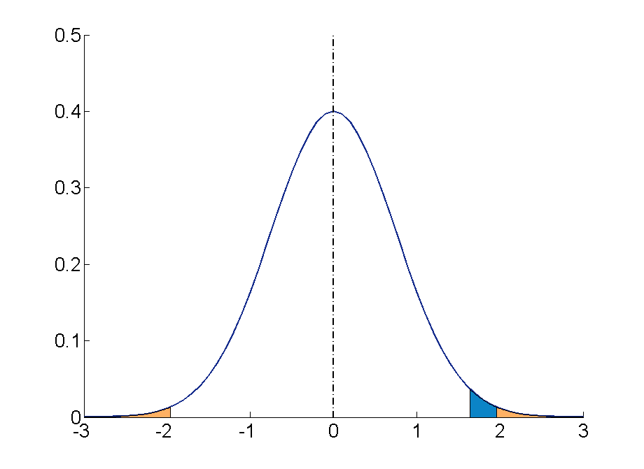
Step 4 : Your sample score of 27 needs to be converted into a Z value. To calculate Z = (27-19)/4= 2 ( check the Converting into Z scores section if you need to review how to do this process)

Step 5 : A ‘Z’ score of 2 is more extreme than the cut off Z of +1.96 (see figure above). The result is significant and, thus, the null hypothesis is rejected.

You can find more examples here:

• Statistics (RMIT Learning Lab)

Some commonly used statistical techniques

Correlation analysis, multiple regression.

• Analysis of variance

Chi-square test for independence

Correlation analysis explores the association between variables . The purpose of correlational analysis is to discover whether there is a relationship between variables, which is unlikely to occur by sampling error. The null hypothesis is that there is no relationship between the two variables. Correlation analysis provides information about:

• The direction of the relationship: positive or negative- given by the sign of the correlation coefficient.
• The strength or magnitude of the relationship between the two variables- given by the correlation coefficient, which varies from 0 (no relationship between the variables) to 1 (perfect relationship between the variables).
• Direction of the relationship.

A positive correlation indicates that high scores on one variable are associated with high scores on the other variable; low scores on one variable are associated with low scores on the second variable . For instance, in the figure below, higher scores on negative affect are associated with higher scores on perceived stress

A negative correlation indicates that high scores on one variable are associated with low scores on the other variable. The graph shows that a person who scores high on perceived stress will probably score low on mastery. The slope of the graph is downwards- as it moves to the right. In the figure below, higher scores on mastery are associated with lower scores on perceived stress.

Fig 2. Negative correlation between two variables. Adapted from Pallant, J. (2013). SPSS survival manual: A step by step guide to data analysis using IBM SPSS (5th ed.). Sydney, Melbourne, Auckland, London: Allen & Unwin

2. The strength or magnitude of the relationship

The strength of a linear relationship between two variables is measured by a statistic known as the correlation coefficient , which varies from 0 to -1, and from 0 to +1. There are several correlation coefficients; the most widely used are Pearson’s r and Spearman’s rho. The strength of the relationship is interpreted as follows:

• Small/weak: r= .10 to .29
• Medium/moderate: r= .30 to .49
• Large/strong: r= .50 to 1

It is important to note that correlation analysis does not imply causality. Correlation is used to explore the association between variables, however, it does not indicate that one variable causes the other. The correlation between two variables could be due to the fact that a third variable is affecting the two variables.

Multiple regression is an extension of correlation analysis. Multiple regression is used to explore the relationship between one dependent variable and a number of independent variables or predictors . The purpose of a multiple regression model is to predict values of a dependent variable based on the values of the independent variables or predictors. For example, a researcher may be interested in predicting students’ academic success (e.g. grades) based on a number of predictors, for example, hours spent studying, satisfaction with studies, relationships with peers and lecturers.

A multiple regression model can be conducted using statistical software (e.g. SPSS). The software will test the significance of the model (i.e. does the model significantly predicts scores on the dependent variable using the independent variables introduced in the model?), how much of the variance in the dependent variable is explained by the model, and the individual contribution of each independent variable.

Example of multiple regression model

From Dunn et al. (2014). Influence of academic self-regulation, critical thinking, and age on online graduate students' academic help-seeking.

In this model, help-seeking is the dependent variable; there are three independent variables or predictors. The coefficients show the direction (positive or negative) and magnitude of the relationship between each predictor and the dependent variable. The model was statistically significant and predicted 13.5% of the variance in help-seeking.

t-Tests are employed to compare the mean score on some continuous variable for two groups . The null hypothesis to be tested is there are no differences between the two groups (e.g. anxiety scores for males and females are not different).

If the significance value of the t-test is equal or less than .05, there is a significant difference in the mean scores on the variable of interest for each of the two groups. If the value is above .05, there is no significant difference between the groups.

t-Tests can be employed to compare the mean scores of two different groups (independent-samples t-test ) or to compare the same group of people on two different occasions ( paired-samples t-test) .

In addition to assessing whether the difference between the two groups is statistically significant, it is important to consider the effect size or magnitude of the difference between the groups. The effect size is given by partial eta squared (proportion of variance of the dependent variable that is explained by the independent variable) and Cohen’s d (difference between groups in terms of standard deviation units).

In this example, an independent samples t-test was conducted to assess whether males and females differ in their perceived anxiety levels. The significance of the test is .004. Since this value is less than .05, we can conclude that there is a statistically significant difference between males and females in their perceived anxiety levels.

Whilst t-tests compare the mean score on one variable for two groups, analysis of variance is used to test more than two groups . Following the previous example, analysis of variance would be employed to test whether there are differences in anxiety scores for students from different disciplines.

Analysis of variance compare the variance (variability in scores) between the different groups (believed to be due to the independent variable) with the variability within each group (believed to be due to chance). An F ratio is calculated; a large F ratio indicates that there is more variability between the groups (caused by the independent variable) than there is within each group (error term). A significant F test indicates that we can reject the null hypothesis; i.e. that there is no difference between the groups.

Again, effect size statistics such as Cohen’s d and eta squared are employed to assess the magnitude of the differences between groups.

In this example, we examined differences in perceived anxiety between students from different disciplines. The results of the Anova Test show that the significance level is .005. Since this value is below .05, we can conclude that there are statistically significant differences between students from different disciplines in their perceived anxiety levels.

Chi-square test for independence is used to explore the relationship between two categorical variables. Each variable can have two or more categories.

For example, a researcher can use a Chi-square test for independence to assess the relationship between study disciplines (e.g. Psychology, Business, Education,…) and help-seeking behaviour (Yes/No). The test compares the observed frequencies of cases with the values that would be expected if there was no association between the two variables of interest. A statistically significant Chi-square test indicates that the two variables are associated (e.g. Psychology students are more likely to seek help than Business students). The effect size is assessed using effect size statistics: Phi and Cramer’s V .

In this example, a Chi-square test was conducted to assess whether males and females differ in their help-seeking behaviour (Yes/No). The crosstabulation table shows the percentage of males of females who sought/didn't seek help. The table 'Chi square tests' shows the significance of the test (Pearson Chi square asymp sig: .482). Since this value is above .05, we conclude that there is no statistically significant difference between males and females in their help-seeking behaviour.

• << Previous: Probability and the normal distribution
• Next: Statistical techniques >>

Asymptotically uniform functions: a single hypothesis which solves two old problems

• Open access
• Published: 05 June 2024

Cite this article

You have full access to this open access article

• J.-P. Gabriel 1 &
• J.-P. Berrut 1  

Explore all metrics

The asymptotic study of a time-dependent function ƒ as the solution of a differential equation often leads to the question of whether its derivative \(f'\) vanishes at infinity. We show that a necessary and sufficient condition for this is that \(f'\) is what may be called asymptotically uniform. We generalize the result to higher order derivatives. We also show that the same property for ƒ itself is also necessary and sufficient for its one-sided improper integrals to exist. The article provides a broad study of such asymptotically uniform functions.

Article PDF

Download to read the full article text

Avoid common mistakes on your manuscript.

T. Andreescu, C. Mortici and M. Tetiva, Mathematical Bridges, Birkhäuser/Springer (New York, 2017).

I. Barbălat, Systèmes d'équations différentielles d'oscillations non linéaires, Rev. Roumaine Math. Pures Appl., 4 (1959), 267-270.

W. A. Coppel, Stability andAsymptotic Behavior of Differential Equations,D.C.Heath and Company (Boston, 1965).

H. T. Croft, A question of limits, Eureca, 20 (1957), 11-13.

P. J. Davis, Interpolation and Approximation, Dover (New York, 1975).

B. Farkas and S.-A. Wegner, Variations on Barbălat's lemma, Amer. Math. Monthly, 123 (2016), 825-830.

B. R. Gelbaum and J. M. H. Olmsted, Counterexamples in Analysis, Holden-Day (San Francisco, 1964).

J. Hadamard, Sur certaines propriétés des trajectoires en Dynamique, J. Math. Pures Appl., 3 (1897), 331-387.

J. Hadamard, Sur le module maximum d'une fonction et de ses dérivées, C. R. Acad. Sci. Paris (1914), 68-72.

G. H. Hardy and J. E. Littlewood, Contributions to the arithmetic theory of series, Proc. London Math. Soc. (2), 11 (1913), 411-478.

F. B. Hildebrand, Introduction to Numerical Analysis, Dover (New York, 1956, 1974).

A. Kneser, Untersuchungen und asymptotische Darstellung der Integrale gewisser Differentialgleichungen bei grossen reellen Werthen des Arguments. I, J. Reine Angew. Math., 116 (1896), 178-212.

E. Landau, Ungleichungen für zweimal differentiierbare Funktionen, Proc. London Math. Soc. (2), 13 (1914), 43-49.

E. Lesigne, On the behavior at infinity of an integrable function, Amer. Math. Monthly, 117 (2010), 175-181.

J. E. Littlewood, The converse of Abel's theorem on power series, Proc. London Math. Soc. (2), 9 (1910-1911), 434-448.

D. S. Mitrinović, J. E. Pečarić and A. M. Fink, Inequalities Involving Functions and their Integrals and Derivatives, Kluwer (Dordrecht, 1991).

P. Müllhaupt, Introduction à l'Analyse et à la Commande des Systèmes Non Liné-aires, Presses Polytechniques et Universitaires Romandes (Lausanne, 2009).

T.-L. T. Rădulescu, V. D. Rădulescu and T. Andreescu, Problems in Real Analysis: Advanced Calculus on the Real Axis, Springer (New York, 2009).

H. R. Thieme, Mathematics in Population Biology, Princeton University Press (2003).

A. C. M. van Rooij and W. H. Schikhof, A Second Course on Real Functions, Cambridge University Press (1982).

Download references

Acknowledgement

The authors are grateful to the reviewer for his many suggestions, on the form as well as with certain theorems and proofs, which have considerably improved this work.

Author information

Authors and affiliations.

Département de Mathématiques, Université de Fribourg, Pérolles, CH-1700, Fribourg, Switzerland

J.-P. Gabriel & J.-P. Berrut

You can also search for this author in PubMed   Google Scholar

Corresponding author

Correspondence to J.-P. Berrut .

Rights and permissions

Open Access This article is licensed under a Creative Commons Attribution 4.0 International License, which permits use, sharing, adaptation, distribution and reproduction in any medium or format, as long as you give appropriate credit to the original author(s) and the source, provide a link to the Creative Commons licence, and indicate if changes were made. The images or other third party material in this article are included in the article's Creative Commons licence, unless indicated otherwise in a credit line to the material. If material is not included in the article's Creative Commons licence and your intended use is not permitted by statutory regulation or exceeds the permitted use, you will need to obtain permission directly from the copyright holder. To view a copy of this licence, visit http://creativecommons.org/licenses/by/4.0/ .

Reprints and permissions

About this article

Gabriel, JP., Berrut, JP. Asymptotically uniform functions: a single hypothesis which solves two old problems. Anal Math (2024). https://doi.org/10.1007/s10476-024-00024-x

Download citation

Received : 17 March 2023

Revised : 09 November 2023

Accepted : 15 December 2023

Published : 05 June 2024

DOI : https://doi.org/10.1007/s10476-024-00024-x

Share this article

Anyone you share the following link with will be able to read this content:

Sorry, a shareable link is not currently available for this article.

Provided by the Springer Nature SharedIt content-sharing initiative

Key words and phrases

• asymptotically uniform function
• vanishing of a derivative at infinity
• vanishing of an integrand at infinity
• Hadamard's lemma
• Barbălat's lemma

Mathematics Subject Classification

• Find a journal
• Publish with us
• Track your research