
Hypothesis Testing and Statistical Significance
This tutorial is a part of the Zero to Data Analyst Bootcamp by Jovian

Hypothesis testing is a technique used by statisticians, scientists and data analysts for measuring whether the results of an experiment are meaningful and reliable. The statistical significance of the results of an experiment is often quantified using a P-value. This tutorial aims to build intuition for hypothesis testing using some real-world examples.
How to Run the Code
The best way to learn the material is to execute the code and experiment with it yourself. This tutorial is an executable Jupyter notebook . You can run this tutorial and experiment with the code examples in a couple of ways: using free online resources (recommended) or on your computer .
Option 1: Running using free online resources (1-click, recommended)
The easiest way to start executing the code is to click the Run button at the top of this page and select Run on Binder . You can also select "Run on Colab" or "Run on Kaggle", but you'll need to create an account on Google Colab or Kaggle to use these platforms.
Option 2: Running on your computer locally
To run the code on your computer locally, you'll need to set up Python , download the notebook and install the required libraries. We recommend using the Conda distribution of Python. Click the Run button at the top of this page, select the Run Locally option, and follow the instructions.
Problem Statement
Let's work through a real-world example to understand how statistical tests are performed:
QUESTION : You're an analyst at the investment firm Capital Ventures, and you're evaluating the company Jovian for a potential investment. The founders of Jovian claim that completing a data science bootcamp offered by Jovian helps you land a data science job faster. A 2020 McKinley report suggests that candidates apply for an average of 37 data science job roles before getting hired. You've surveyed 42 Jovian bootcamp graduates who are now working in data science roles, and compiled data for the number of jobs each one applied to before getting hired: 31, 23, 19, 42, 37, 18, 7, 53, 33, 17, 27, 41, 36, 29, 60, 34, 21, 18, 45, 33, 16, 10, 48, 32, 19, 29, 40, 35, 28, 57, 25, 31, 19, 40, 37, 33, 38, 28, 40, 36, 42, 39 Is there a statistically significant decrease in the number of jobs candidates need to apply to before getting hired if they've completed a bootcamp offered by Jovian?
Have a language expert improve your writing
Run a free plagiarism check in 10 minutes, generate accurate citations for free.
- Knowledge Base
Hypothesis Testing | A Step-by-Step Guide with Easy Examples
Published on November 8, 2019 by Rebecca Bevans . Revised on June 22, 2023.
Hypothesis testing is a formal procedure for investigating our ideas about the world using statistics . It is most often used by scientists to test specific predictions, called hypotheses, that arise from theories.
There are 5 main steps in hypothesis testing:
- State your research hypothesis as a null hypothesis and alternate hypothesis (H o ) and (H a or H 1 ).
- Collect data in a way designed to test the hypothesis.
- Perform an appropriate statistical test .
- Decide whether to reject or fail to reject your null hypothesis.
- Present the findings in your results and discussion section.
Though the specific details might vary, the procedure you will use when testing a hypothesis will always follow some version of these steps.
Table of contents
Step 1: state your null and alternate hypothesis, step 2: collect data, step 3: perform a statistical test, step 4: decide whether to reject or fail to reject your null hypothesis, step 5: present your findings, other interesting articles, frequently asked questions about hypothesis testing.
After developing your initial research hypothesis (the prediction that you want to investigate), it is important to restate it as a null (H o ) and alternate (H a ) hypothesis so that you can test it mathematically.
The alternate hypothesis is usually your initial hypothesis that predicts a relationship between variables. The null hypothesis is a prediction of no relationship between the variables you are interested in.
- H 0 : Men are, on average, not taller than women. H a : Men are, on average, taller than women.
Receive feedback on language, structure, and formatting
Professional editors proofread and edit your paper by focusing on:
- Academic style
- Vague sentences
- Style consistency
See an example

For a statistical test to be valid , it is important to perform sampling and collect data in a way that is designed to test your hypothesis. If your data are not representative, then you cannot make statistical inferences about the population you are interested in.
There are a variety of statistical tests available, but they are all based on the comparison of within-group variance (how spread out the data is within a category) versus between-group variance (how different the categories are from one another).
If the between-group variance is large enough that there is little or no overlap between groups, then your statistical test will reflect that by showing a low p -value . This means it is unlikely that the differences between these groups came about by chance.
Alternatively, if there is high within-group variance and low between-group variance, then your statistical test will reflect that with a high p -value. This means it is likely that any difference you measure between groups is due to chance.
Your choice of statistical test will be based on the type of variables and the level of measurement of your collected data .
- an estimate of the difference in average height between the two groups.
- a p -value showing how likely you are to see this difference if the null hypothesis of no difference is true.
Based on the outcome of your statistical test, you will have to decide whether to reject or fail to reject your null hypothesis.
In most cases you will use the p -value generated by your statistical test to guide your decision. And in most cases, your predetermined level of significance for rejecting the null hypothesis will be 0.05 – that is, when there is a less than 5% chance that you would see these results if the null hypothesis were true.
In some cases, researchers choose a more conservative level of significance, such as 0.01 (1%). This minimizes the risk of incorrectly rejecting the null hypothesis ( Type I error ).
The results of hypothesis testing will be presented in the results and discussion sections of your research paper , dissertation or thesis .
In the results section you should give a brief summary of the data and a summary of the results of your statistical test (for example, the estimated difference between group means and associated p -value). In the discussion , you can discuss whether your initial hypothesis was supported by your results or not.
In the formal language of hypothesis testing, we talk about rejecting or failing to reject the null hypothesis. You will probably be asked to do this in your statistics assignments.
However, when presenting research results in academic papers we rarely talk this way. Instead, we go back to our alternate hypothesis (in this case, the hypothesis that men are on average taller than women) and state whether the result of our test did or did not support the alternate hypothesis.
If your null hypothesis was rejected, this result is interpreted as “supported the alternate hypothesis.”
These are superficial differences; you can see that they mean the same thing.
You might notice that we don’t say that we reject or fail to reject the alternate hypothesis . This is because hypothesis testing is not designed to prove or disprove anything. It is only designed to test whether a pattern we measure could have arisen spuriously, or by chance.
If we reject the null hypothesis based on our research (i.e., we find that it is unlikely that the pattern arose by chance), then we can say our test lends support to our hypothesis . But if the pattern does not pass our decision rule, meaning that it could have arisen by chance, then we say the test is inconsistent with our hypothesis .
If you want to know more about statistics , methodology , or research bias , make sure to check out some of our other articles with explanations and examples.
- Normal distribution
- Descriptive statistics
- Measures of central tendency
- Correlation coefficient
Methodology
- Cluster sampling
- Stratified sampling
- Types of interviews
- Cohort study
- Thematic analysis
Research bias
- Implicit bias
- Cognitive bias
- Survivorship bias
- Availability heuristic
- Nonresponse bias
- Regression to the mean
Hypothesis testing is a formal procedure for investigating our ideas about the world using statistics. It is used by scientists to test specific predictions, called hypotheses , by calculating how likely it is that a pattern or relationship between variables could have arisen by chance.
A hypothesis states your predictions about what your research will find. It is a tentative answer to your research question that has not yet been tested. For some research projects, you might have to write several hypotheses that address different aspects of your research question.
A hypothesis is not just a guess — it should be based on existing theories and knowledge. It also has to be testable, which means you can support or refute it through scientific research methods (such as experiments, observations and statistical analysis of data).
Null and alternative hypotheses are used in statistical hypothesis testing . The null hypothesis of a test always predicts no effect or no relationship between variables, while the alternative hypothesis states your research prediction of an effect or relationship.
Cite this Scribbr article
If you want to cite this source, you can copy and paste the citation or click the “Cite this Scribbr article” button to automatically add the citation to our free Citation Generator.
Bevans, R. (2023, June 22). Hypothesis Testing | A Step-by-Step Guide with Easy Examples. Scribbr. Retrieved June 11, 2024, from https://www.scribbr.com/statistics/hypothesis-testing/
Is this article helpful?

Rebecca Bevans
Other students also liked, choosing the right statistical test | types & examples, understanding p values | definition and examples, what is your plagiarism score.
If you're seeing this message, it means we're having trouble loading external resources on our website.
If you're behind a web filter, please make sure that the domains *.kastatic.org and *.kasandbox.org are unblocked.
To log in and use all the features of Khan Academy, please enable JavaScript in your browser.
Unit 12: Significance tests (hypothesis testing)
About this unit.
Significance tests give us a formal process for using sample data to evaluate the likelihood of some claim about a population value. Learn how to conduct significance tests and calculate p-values to see how likely a sample result is to occur by random chance. You'll also see how we use p-values to make conclusions about hypotheses.
The idea of significance tests
- Simple hypothesis testing (Opens a modal)
- Idea behind hypothesis testing (Opens a modal)
- Examples of null and alternative hypotheses (Opens a modal)
- P-values and significance tests (Opens a modal)
- Comparing P-values to different significance levels (Opens a modal)
- Estimating a P-value from a simulation (Opens a modal)
- Using P-values to make conclusions (Opens a modal)
- Simple hypothesis testing Get 3 of 4 questions to level up!
- Writing null and alternative hypotheses Get 3 of 4 questions to level up!
- Estimating P-values from simulations Get 3 of 4 questions to level up!
Error probabilities and power
- Introduction to Type I and Type II errors (Opens a modal)
- Type 1 errors (Opens a modal)
- Examples identifying Type I and Type II errors (Opens a modal)
- Introduction to power in significance tests (Opens a modal)
- Examples thinking about power in significance tests (Opens a modal)
- Consequences of errors and significance (Opens a modal)
- Type I vs Type II error Get 3 of 4 questions to level up!
- Error probabilities and power Get 3 of 4 questions to level up!
Tests about a population proportion
- Constructing hypotheses for a significance test about a proportion (Opens a modal)
- Conditions for a z test about a proportion (Opens a modal)
- Reference: Conditions for inference on a proportion (Opens a modal)
- Calculating a z statistic in a test about a proportion (Opens a modal)
- Calculating a P-value given a z statistic (Opens a modal)
- Making conclusions in a test about a proportion (Opens a modal)
- Writing hypotheses for a test about a proportion Get 3 of 4 questions to level up!
- Conditions for a z test about a proportion Get 3 of 4 questions to level up!
- Calculating the test statistic in a z test for a proportion Get 3 of 4 questions to level up!
- Calculating the P-value in a z test for a proportion Get 3 of 4 questions to level up!
- Making conclusions in a z test for a proportion Get 3 of 4 questions to level up!
Tests about a population mean
- Writing hypotheses for a significance test about a mean (Opens a modal)
- Conditions for a t test about a mean (Opens a modal)
- Reference: Conditions for inference on a mean (Opens a modal)
- When to use z or t statistics in significance tests (Opens a modal)
- Example calculating t statistic for a test about a mean (Opens a modal)
- Using TI calculator for P-value from t statistic (Opens a modal)
- Using a table to estimate P-value from t statistic (Opens a modal)
- Comparing P-value from t statistic to significance level (Opens a modal)
- Free response example: Significance test for a mean (Opens a modal)
- Writing hypotheses for a test about a mean Get 3 of 4 questions to level up!
- Conditions for a t test about a mean Get 3 of 4 questions to level up!
- Calculating the test statistic in a t test for a mean Get 3 of 4 questions to level up!
- Calculating the P-value in a t test for a mean Get 3 of 4 questions to level up!
- Making conclusions in a t test for a mean Get 3 of 4 questions to level up!
More significance testing videos
- Hypothesis testing and p-values (Opens a modal)
- One-tailed and two-tailed tests (Opens a modal)
- Z-statistics vs. T-statistics (Opens a modal)
- Small sample hypothesis test (Opens a modal)
- Large sample proportion hypothesis testing (Opens a modal)
- Docs »
- Welcome to Jovian!
- Edit on GitHub
Welcome to Jovian! 
Jovian is a platform that helps data scientists and ML engineers:
Track & reproduce data science projects
Collaborate easily with friends/colleagues, and
Automate repetitive tasks in their day-to-day workflow.
Getting Started 
Learn more about installing Jovian python library and some of the core features of Jovian.
Run this command in your terminal:
DSpace JSPUI
Egyankosh preserves and enables easy and open access to all types of digital content including text, images, moving images, mpegs and data sets.
- IGNOU Self Learning Material (SLM)
- 03. School of Sciences (SOS)
- Diploma / Post Graduate Diploma Programmes
- Post-Graduate Diploma in Applied Statistics (PGDAST)
- MST-004 Statistical Inference
- Block-3 Testing of Hypothesis
| Title: | Unit-9 Concepts of Testing of Hypothesis |
| Contributors: | |
| Issue Date: | 2017 |
| Publisher: | IGNOU |
| URI: | |
| Appears in Collections: | |
| File | Description | Size | Format | |
|---|---|---|---|---|
| 433.61 kB | Adobe PDF | |
Items in eGyanKosh are protected by copyright, with all rights reserved, unless otherwise indicated.

Chapter 9 Hypothesis Testing
- KEY TERMS AND CONCEPTS
- SCIENTISTS IN ACTION

What is a Hypothesis?

Null and Alternative Hypotheses

Critical Region, Critical Values and Significance Level

Types of Hypothesis Testing

Decision Making: P -value Method

Decision Making: Traditional Method

Hypothesis: Accept or Fail to Reject?

Errors In Hypothesis Tests

Testing a Claim about Population Proportion

Testing a Claim about Mean: Known Population SD

Testing a Claim about Mean: Unknown Population SD

Testing a Claim about Standard Deviation

Novel Object Recognition and Object Location Behavioral Testing in Mice on a Budget

Use of Galvanic Skin Responses, Salivary Biomarkers, and Self-reports to Assess Undergraduate Student Performance During a Laboratory Exam Activity

Meta-analysis of Voxel-Based Neuroimaging Studies using Seed-based d Mapping with Permutation of Subject Images (SDM-PSI)
Get cutting-edge science videos from j o ve sent straight to your inbox every month..
mktb-description
We use cookies to enhance your experience on our website.
By continuing to use our website or clicking “Continue”, you are agreeing to accept our cookies.
Thank you for visiting nature.com. You are using a browser version with limited support for CSS. To obtain the best experience, we recommend you use a more up to date browser (or turn off compatibility mode in Internet Explorer). In the meantime, to ensure continued support, we are displaying the site without styles and JavaScript.
- View all journals
- Explore content
- About the journal
- Publish with us
- Sign up for alerts
- Published: 06 June 2024
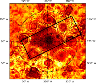
Frontogenesis at Jovian high latitudes
- Lia Siegelman ORCID: orcid.org/0000-0003-3330-082X 1 &
- Patrice Klein ORCID: orcid.org/0000-0002-3089-3896 2 , 3
Nature Physics ( 2024 ) Cite this article
173 Accesses
168 Altmetric
Metrics details
- Fluid dynamics
- Giant planets
Frontogenesis is the process by which fronts, separating fluids of different temperatures, are generated in the terrestrial atmosphere and oceans. It is of interest to consider whether this process appears in other planetary atmospheres. Here we analyse infra-red images taken by the Juno spacecraft at the Jovian poles and reveal ubiquitous vortices with a diameter of hundreds to thousands of kilometres and filaments with a width of tens of kilometres embedded in between the vortices. Our analysis shows that the filaments are dynamically active, reminiscent of terrestrial frontogenesis. Furthermore, our results indicate that Jovian frontogenesis acts in concert with moist convection, with the former mechanism favouring the development of cyclones and the latter the development of anti-cyclones. Even though moist convection is the main driver, frontogenesis accounts for a quarter of the total transfer of potential to kinetic energy, enhancing the upscale transfer of energy to larger vortices. Frontogenesis contributes 40% to the vertical heat transport, efficiently redistributing heat from Jupiter’s interior to its tropopause. This study highlights the broad range of interacting scales from tens to thousands of kilometres and the diverse physical mechanisms active at Jovian high latitudes.
This is a preview of subscription content, access via your institution
Access options
Access Nature and 54 other Nature Portfolio journals
Get Nature+, our best-value online-access subscription
24,99 € / 30 days
cancel any time
Subscribe to this journal
Receive 12 print issues and online access
195,33 € per year
only 16,28 € per issue
Buy this article
- Purchase on Springer Link
- Instant access to full article PDF
Prices may be subject to local taxes which are calculated during checkout
Moist convection drives an upscale energy transfer at Jovian high latitudes

Enhanced upward heat transport at deep submesoscale ocean fronts

Global upper-atmospheric heating on Jupiter by the polar aurorae
Data availability.
JIRAM data are available at the Planetary Data System (PDS) online ( https://atmos.nmsu.edu/PDS/data/PDS4/juno_jiram_bundle/data_calibrated/ ). Data products used in this study are the same as used in ref. 4 . They include calibrated, geometrically controlled, radiance data mapped onto an orthographic projection centred on the north pole and velocity vectors derived from the radiance data. Brightness maps and velocity vectors can be found in the supplementary data sets of ref. 4 .
Code availability
The code is available at https://github.com/liasiegelman/JIRAM/blob/main/frontogenesis.py .
Bolton, S. J. et al. Jupiter’s interior and deep atmosphere: the initial pole-to-pole passes with the Juno spacecraft. Science 356 , 821–825 (2017).
Article ADS Google Scholar
Adriani, A. et al. Clusters of cyclones encircling Jupiter’s poles. Nature 555 , 216–219 (2018).
Moriconi, M. et al. Turbulence power spectra in regions surrounding Jupiter’s south polar cyclones from Juno/JIRAM. J. Geophys. Res. Planets 125 , e2019JE006096 (2020).
Siegelman, L. et al. Moist convection drives an upscale energy transfer at jovian high latitudes. Nat. Phys. 18 , 357–361 (2022).
Article Google Scholar
Siegelman, L., Young, W. R. & Ingersoll, A. P. Polar vortex crystals: emergence and structure. Proc. Natl Acad. Sci. USA 119 , e2120486119 (2022).
Article MathSciNet Google Scholar
Hoskins, B. J. & Bretherton, F. P. Atmospheric frontogenesis models: mathematical formulation and solution. J. Atmos. Sci. 29 , 11–27 (1972).
2.0.CO;2" data-track-item_id="10.1175/1520-0469(1972)029 2.0.CO;2" data-track-value="article reference" data-track-action="article reference" href="https://doi.org/10.1175%2F1520-0469%281972%29029%3C0011%3AAFMMFA%3E2.0.CO%3B2" aria-label="Article reference 6" data-doi="10.1175/1520-0469(1972)029 2.0.CO;2">Article ADS Google Scholar
Hakim, G. & Keyser, D. Canonical frontal circulation patterns in terms of Green’s functions for the Sawyer–Eliassen equation. Q. J. R. Meteorol. Soc. 127 , 1795–1814 (2001).
ADS Google Scholar
Capet, X., Klein, P., Hua, B. L., Lapeyre, G. & Mcwilliams, J. C. Surface kinetic energy transfer in surface quasi-geostrophic flows. J. Fluid Mech. 604 , 165–174 (2008).
Adriani, A. et al. Two-year observations of the Jupiter polar regions by JIRAM on board Juno. J. Geophys. Res. Planets 125 , e2019JE006098 (2020).
Lapeyre, G. Surface quasi-geostrophy. Fluids 2 , 7 (2017).
Juckes, M. Quasigeostrophic dynamics of the tropopause. J. Atmos. Sci. 51 , 2756–2768 (1994).
2.0.CO;2" data-track-item_id="10.1175/1520-0469(1994)051 2.0.CO;2" data-track-value="article reference" data-track-action="article reference" href="https://doi.org/10.1175%2F1520-0469%281994%29051%3C2756%3AQDOTT%3E2.0.CO%3B2" aria-label="Article reference 11" data-doi="10.1175/1520-0469(1994)051 2.0.CO;2">Article ADS Google Scholar
Juckes, M. Instability of surface and upper-tropospheric shear lines. J. Atmos. Sci. 52 , 3247–3262 (1995).
2.0.CO;2" data-track-item_id="10.1175/1520-0469(1995)052 2.0.CO;2" data-track-value="article reference" data-track-action="article reference" href="https://doi.org/10.1175%2F1520-0469%281995%29052%3C3247%3AIOSAUT%3E2.0.CO%3B2" aria-label="Article reference 12" data-doi="10.1175/1520-0469(1995)052 2.0.CO;2">Article ADS MathSciNet Google Scholar
Hakim, G. J., Snyder, C. & Muraki, D. J. A new surface model for cyclone–anticyclone asymmetry. J. Atmos. Sci. 59 , 2405–2420 (2002).
2.0.CO;2" data-track-item_id="10.1175/1520-0469(2002)059 2.0.CO;2" data-track-value="article reference" data-track-action="article reference" href="https://doi.org/10.1175%2F1520-0469%282002%29059%3C2405%3AANSMFC%3E2.0.CO%3B2" aria-label="Article reference 13" data-doi="10.1175/1520-0469(2002)059 2.0.CO;2">Article ADS MathSciNet Google Scholar
Lapeyre, G. & Klein, P. Impact of the small-scale elongated filaments on the oceanic vertical pump. J. Mar. Res. 64 , 835–851 (2006).
Lapeyre, G. & Klein, P. Dynamics of the upper oceanic layers in terms of surface quasigeostrophy theory. J. Phys. Oceanogr. 36 , 165–176 (2006).
Article ADS MathSciNet Google Scholar
Young, R. M. & Read, P. L. Forward and inverse kinetic energy cascades in Jupiter’s turbulent weather layer. Nat. Phys. 13 , 1135–1140 (2017).
Read, P. L. The dynamics of Jupiter’s and Saturn’s weather layers: a synthesis after Cassini and Juno. Annu. Rev. Fluid Mech. 56 , 271–293 (2023).
Achterberg, R. K. & Ingersoll, A. P. A normal-mode approach to jovian atmospheric dynamics. J. Atmos. Sci. 46 , 2448–2462 (1989).
2.0.CO;2" data-track-item_id="10.1175/1520-0469(1989)046 2.0.CO;2" data-track-value="article reference" data-track-action="article reference" href="https://doi.org/10.1175%2F1520-0469%281989%29046%3C2448%3AANMATJ%3E2.0.CO%3B2" aria-label="Article reference 18" data-doi="10.1175/1520-0469(1989)046 2.0.CO;2">Article ADS Google Scholar
Young, R. M., Read, P. L. & Wang, Y. Simulating jupiter’s weather layer. Part I: jet spin-up in a dry atmosphere. Icarus 326 , 225–252 (2019).
Shcherbina, A. Y. et al. Statistics of vertical vorticity, divergence, and strain in a developed submesoscale turbulence field. Geophys. Res. Lett. 40 , 4706–4711 (2013).
Balwada, D., Xiao, Q., Smith, S., Abernathey, R. & Gray, A. R. Vertical fluxes conditioned on vorticity and strain reveal submesoscale ventilation. J. Phys. Oceanogr. 51 , 2883–2901 (2021).
Hoskins, B. J. The mathematical theory of frontogenesis. Annu. Rev. Fluid Mech. 14 , 131–151 (1982).
Ingersoll, A., Gierasch, P., Banfield, D., Vasavada, A. & Team, G. I. Moist convection as an energy source for the large-scale motions in Jupiter’s atmosphere. Nature 403 , 630–632 (2000).
Gierasch, P. et al. Observation of moist convection in Jupiter’s atmosphere. Nature 403 , 628–630 (2000).
Vallis, G. K. Atmospheric and Oceanic Fluid Dynamics (Cambridge Univ. Press, 2017).
O’Neill, M. E., Emanuel, K. A. & Flierl, G. R. Polar vortex formation in giant-planet atmospheres due to moist convection. Nat. Geosci. 8 , 523–526 (2015).
Okubo, A. Horizontal dispersion of floatable particles in the vicinity of velocity singularities such as convergences. Deep Sea Res. Oceanogr. Abs. 17 , 445–454 (1970).
Weiss, J. The dynamics of enstrophy transfer in two-dimensional hydrodynamics. Physica D 48 , 273–294 (1991).
O’Neill, M. E., Emanuel, K. A. & Flierl, G. R. Weak jets and strong cyclones: shallow-water modeling of giant planet polar caps. J. Atmos. Sci. 73 , 1841–1855 (2016).
Hueso, R. & Sánchez-Lavega, A. A three-dimensional model of moist convection for the giant planets: the Jupiter case. Icarus 151 , 257–274 (2001).
Hueso, R., Sánchez-Lavega, A. & Guillot, T. A model for large-scale convective storms in Jupiter. J. Geophys. Res. Planets 107 , 5-1–5-11 (2002).
Sawyer, J. S. The vertical circulation at meteorological fronts and its relation to frontogenesis. Proc. R. Soc. London A 234 , 346–362 (1956).
Held, I. M., Pierrehumbert, R. T., Garner, S. T. & Swanson, K. L. Surface quasi-geostrophic dynamics. J. Fluid Mech. 282 , 1–20 (1995).
Thomas, L. N., Tandon, A. & Mahadevan, A. in Ocean Modeling in an Eddying Regime Vol. 177 (eds Thomas, L. N. et al.) 17–38 (American Geophysical Union, 2008).
Klein, P. & Lapeyre, G. The oceanic vertical pump induced by mesoscale and submesoscale turbulence. Annu. Rev. Mar. Sci. 1 , 351–375 (2009).
Pirraglia, J. Meridional energy balance of Jupiter. Icarus 59 , 169–176 (1984).
Li, L. et al. Less absorbed solar energy and more internal heat for Jupiter. Nat. Commun. 9 , 3709 (2018).
Adriani, A. et al. JIRAM, the Jovian infrared auroral mapper. Space Sci. Rev. 213 , 393–446 (2017).
Ferrari, R. A frontal challenge for climate models. Science 332 , 316–317 (2011).
Wolfe, C., Cessi, P., McClean, J. & Maltrud, M. Vertical heat transport in eddying ocean models. Geophys. Res. Lett. 35 , L23605 (2008).
Su, Z., Wang, J., Klein, P., Thompson, A. F. & Menemenlis, D. Ocean submesoscales as a key component of the global heat budget. Nat. Commun. 9 , 775 (2018).
Nastrom, G. & Gage, K. S. A climatology of atmospheric wavenumber spectra of wind and temperature observed by commercial aircraft. J. Atmos. Sci. 42 , 950–960 (1985).
2.0.CO;2" data-track-item_id="10.1175/1520-0469(1985)042 2.0.CO;2" data-track-value="article reference" data-track-action="article reference" href="https://doi.org/10.1175%2F1520-0469%281985%29042%3C0950%3AACOAWS%3E2.0.CO%3B2" aria-label="Article reference 42" data-doi="10.1175/1520-0469(1985)042 2.0.CO;2">Article ADS Google Scholar
Tulloch, R. & Smith, K. A theory for the atmospheric energy spectrum: depth-limited temperature anomalies at the tropopause. Proc. Natl Acad. Sci. USA 103 , 14690–14694 (2006).
Waite, M. L. & Snyder, C. Mesoscale energy spectra of moist baroclinic waves. J. Atmos. Sci. 70 , 1242–1256 (2013).
Burgess, B. H., Erler, A. R. & Shepherd, T. G. The troposphere-to-stratosphere transition in kinetic energy spectra and nonlinear spectral fluxes as seen in ECMWF analyses. J. Atmos. Sci. 70 , 669–687 (2013).
Hamilton, K., Takahashi, Y. O. & Ohfuchi, W. Mesoscale spectrum of atmospheric motions investigated in a very fine resolution global general circulation model. J. Geophys. Res. Atmos. 113 , 110–129 (2008).
Rubio, A. M., Julien, K., Knobloch, E. & Weiss, J. B. Upscale energy transfer in three-dimensional rapidly rotating turbulent convection. Phys. Rev. Lett. 112 , 144501 (2014).
Julien, K., Rubio, A. M., Grooms, I. & Knobloch, E. Statistical and physical balances in low rossby number Rayleigh–Bénard convection. Geophys. Astrophys. Fluid Dyn. 106 , 392–428 (2012).
Favier, B., Silvers, L. & Proctor, M. Inverse cascade and symmetry breaking in rapidly rotating Boussinesq convection. Phys. Fluids 26 , 096605 (2014).
Guervilly, C., Hughes, D. W. & Jones, C. A. Large-scale-vortex dynamos in planar rotating convection. J. Fluid Mech. 815 , 333–360 (2017).
Ingersoll, A. P. et al. Vorticity and divergence at scales down to 200 km within and around the polar cyclones of Jupiter. Nat. Astron. 6 , 1280–1286 (2022).
Orszag, S. A. Numerical simulation of incompressible flows within simple boundaries: accuracy. J. Fluid Mech. 49 , 75–112 (1971).
Charney, J. G. Geostrophic turbulence. J. Atmos. Sci. 28 , 1087–1095 (1971).
2.0.CO;2" data-track-item_id="10.1175/1520-0469(1971)028 2.0.CO;2" data-track-value="article reference" data-track-action="article reference" href="https://doi.org/10.1175%2F1520-0469%281971%29028%3C1087%3AGT%3E2.0.CO%3B2" aria-label="Article reference 53" data-doi="10.1175/1520-0469(1971)028 2.0.CO;2">Article ADS Google Scholar
Blumen, W. Uniform potential vorticity flow: part I. Theory of wave interactions and two-dimensional turbulence. J. Atmos. Sci. 35 , 774–783 (1978).
2.0.CO;2" data-track-item_id="10.1175/1520-0469(1978)035 2.0.CO;2" data-track-value="article reference" data-track-action="article reference" href="https://doi.org/10.1175%2F1520-0469%281978%29035%3C0774%3AUPVFPI%3E2.0.CO%3B2" aria-label="Article reference 54" data-doi="10.1175/1520-0469(1978)035 2.0.CO;2">Article ADS Google Scholar
Lapeyre, G. What vertical mode does the altimeter reflect? On the decomposition in baroclinic modes and on a surface-trapped mode. J. Phys. Oceanogr. 39 , 2857–2874 (2009).
Holton, J. R. (ed.) An Introduction to Dynamic Meteorology Vol. 88 (Elsevier Academic, 2004).
Hua, B. L., McWilliams, J. C. & Klein, P. Lagrangian accelerations in geostrophic turbulence. J. Fluid Mech. 366 , 87–108 (1998).
Download references
Acknowledgements
We thank T. Ewald for processing the infra-red images taken by JIRAM used in this study and W. Young for insightful discussions. L.S. is supported by the National Science Foundation (OCE-1657041). P.K. acknowledges funding from JPL/NASA.
Author information
Authors and affiliations.
Scripps Institution of Oceanography, University of California San Diego, La Jolla, CA, USA
Lia Siegelman
Division of Geological and Planetary Sciences, California Institute of Technology, Pasadena, CA, USA
Patrice Klein
LMD/IPSL, École Normale Supérieure, Université PSL, CNRS, Sorbonne Université, École Polytechnique, Paris, France
You can also search for this author in PubMed Google Scholar
Contributions
L.S. and P.K. led the data analysis and data interpretation and wrote the manuscript.
Corresponding author
Correspondence to Lia Siegelman .
Ethics declarations
Competing interests.
The authors declare no competing interests.
Peer review
Peer review information.
Nature Physics thanks Ricardo Hueso Alonso and the other, anonymous, reviewer(s) for their contribution to the peer review of this work.
Additional information
Publisher’s note Springer Nature remains neutral with regard to jurisdictional claims in published maps and institutional affiliations.
Extended data
Extended data fig. 1 cumulative integrals of χ..
Same as Fig. 4 for \(\tilde{{\chi }^{+}}/\overline{{\chi }^{+}}\) (red curve) and \(\tilde{{\chi }^{-}}/\overline{{\chi }^{-}}\) (blue curve). The dotted line shows the fractional area as a function of \({{{{\rm{d}}}}}_{\max }/{{{\rm{d}}}}\) , with d the vorticity-strain JDF and \({{{{\rm{d}}}}}_{\max }\) its maximum, χ + are updrafts and χ − downdrafts. \(\overline{{\chi }^{+}}\) and \(\overline{{\chi }^{-}}\) have equal magnitude of 0.3 f . The shaded envelopes indicate the range of results obtained with the different low-pass Butterworth filters (see error section in the Methods ). This figure confirms the asymmetry observed in the strain-vorticity space (Fig. 3c ). For instance, scales larger than 230 km, which occupy half of the domain, capture a little over 50% of the χ + but only 10% of the χ − . Similarly, scales smaller than 150 km, which occupy twenty percent of the domain, capture almost 60% of the χ − but only about 20% of χ + . In summary, positive divergence is localized in a large fraction of the physical space and corresponds to large length scales, whereas negative divergence is scattered throughout the domain, occupies a small fraction of the physical space, and corresponds to small length scales.
Extended Data Fig. 2 Spectrum of ζ and χ.
Wavenumber spectrum of vorticity ζ used in this paper (thick black curve) and wavenumber spectra of divergence χ (thin colored curves) derived after filtering the wind velocities derived from feature tracking with a low-pass Butterworth filter of order n and wavelength cutoff w cutoff . The spectra of ζ is used a an upper bound for the derivation of χ . χ used in the study corresponds to the low-pass Butterworth filter of order 1 and cutoff wavelength of 250 km (green curve, see error section in the Methods ).
Extended Data Fig. 3 Error propagation and sensitivity analysis.
Error propagation analysis in wind velocities derived from feature tracking. Each panel shows the weighted JDF of χ /f in vorticity-strain space, with χ the divergence derived after application of a low-pass Butterworth of order n and cutoff wavelength w cutoff and f the Coriolis parameter. The dashed lines are the ∣ ζ ∣ = σ lines, with ζ the vorticity and σ strain. a ) n = 5, w cutoff = 50 km; b ) n = 5, w cutoff = 100 km; c ) n = 1, w cutoff = 250 km, d ) n = 1, w cutoff = 300 km, e ) n = 2, w cutoff = 300 km, f ) n = 2, w cutoff = 500 km. Panel c corresponds to Fig. 3c in the main text. The dispersion in panel a indicates that scales ≤ 50 km contain too much noise. All other panels yield comparable results indicating that the effective resolution of the divergence is between 50 and 100 km (see error section in the Methods for more details).
Rights and permissions
Springer Nature or its licensor (e.g. a society or other partner) holds exclusive rights to this article under a publishing agreement with the author(s) or other rightsholder(s); author self-archiving of the accepted manuscript version of this article is solely governed by the terms of such publishing agreement and applicable law.
Reprints and permissions
About this article
Cite this article.
Siegelman, L., Klein, P. Frontogenesis at Jovian high latitudes. Nat. Phys. (2024). https://doi.org/10.1038/s41567-024-02516-x
Download citation
Received : 16 May 2023
Accepted : 17 April 2024
Published : 06 June 2024
DOI : https://doi.org/10.1038/s41567-024-02516-x
Share this article
Anyone you share the following link with will be able to read this content:
Sorry, a shareable link is not currently available for this article.
Provided by the Springer Nature SharedIt content-sharing initiative
Quick links
- Explore articles by subject
- Guide to authors
- Editorial policies
Sign up for the Nature Briefing newsletter — what matters in science, free to your inbox daily.

HypothesisTests package
This package implements several hypothesis tests in Julia.
- Confidence interval
- Parametric tests
- Power divergence test
- Pearson chi-squared test
- Multinomial likelihood ratio test
- One-way ANOVA Test
- Levene's Test
- Brown-Forsythe Test
- Nonparametric tests
- Anderson-Darling test
- Binomial test
- Fisher exact test
- Kolmogorov-Smirnov test
- Kruskal-Wallis rank sum test
- Mann-Whitney U test
- Wald-Wolfowitz independence test
- Wilcoxon signed rank test
- Permutation test
- Fligner-Killeen test
- Time series tests
- Durbin-Watson test
- Box-Pierce and Ljung-Box tests
- Breusch-Godfrey test
- Jarque-Bera test
- Augmented Dickey-Fuller test
- Clark-West test
- Diebold-Mariano test
- Multivariate tests
- Hotelling's $T^2$ test
- Equality of covariance matrices
- Correlation and partial correlation test
Theme documenter-light documenter-dark
This document was generated with Documenter.jl version 0.27.24 on Wednesday 31 May 2023 . Using Julia version 1.9.0.
Assignment - Evaluating A/B Tests
This assignment is part of the Zero to Data Analyst Bootcamp by Jovian .
As you go through this notebook, you will find the symbol ??? in certain places. To complete this assignment, you must replace all the ??? with appropriate values, expressions, or statements to ensure that the notebook runs properly end-to-end.
- Make sure to run all the code cells in order. Otherwise, you may get errors like NameError for undefined variables.
- Do not change variable names, delete cells, or disturb other existing code. It may cause problems during evaluation.
- In some cases, you may need to add some code cells or new statements before or after the line of code containing the ??? .
- Since you'll be using a temporary online service for code execution, save your work by running jovian.commit at regular intervals.
- Questions marked (Optional) will not be considered for evaluation and can be skipped. They are for your learning.
- If you are stuck, you can ask for help on the bootcamp Slack group. Post errors, ask for hints, and help others, but please don't share the complete solution code on Slack to give others a chance to write the code themselves.
- There are some tests included with this notebook to help you test your implementation. However, after submission, your code will be tested with some hidden test cases. Make sure to test your code exhaustively to cover all edge cases.
Important Links:
Make a submission here: https://jovian.ai/learn/zero-to-data-analyst-bootcamp/assignment/assignment-3-evaluating-a-b-tests
Hypothesis testing tutorial: https://jovian.ai/learn/zero-to-data-analyst-bootcamp/lesson/hypothesis-testing-statistical-signficance
How to Run the Code and Save Your Work
Option 1: Running using free online resources (1-click, recommended) : Click the Run button at the top of this page and select Run on Binder . You can also select "Run on Colab" or "Run on Kaggle", but you'll need to create an account on Google Colab or Kaggle to use these platforms.
Option 2: Running on your computer locally : To run the code on your computer locally, you'll need to set up Python & Conda , download the notebook and install the required libraries. Click the Run button at the top of this page, select the Run Locally option, and follow the instructions.
Saving your work : You can save a snapshot of the assignment to your Jovian profile, so that you can access it later and continue your work. Keep saving your work by running jovian.commit from time to time.
IMAGES
VIDEO
COMMENTS
Hypothesis testing is a technique used by statisticians, scientists and data analysts for measuring whether the results of an experiment are meaningful and reliable. The statistical significance of the results of an experiment is often quantified using a P-value. This tutorial aims to build intuition for hypothesis testing using some real-world ...
Solution: Assuming the null hypothesis H_0 H 0 is true. Throwing a coin is the perfect example of a bernoulli distribution. Which is why we can directly use the formula for standard deviation. \sigma = \sqrt {p (1-p)} σ = p(1 −p) Now, let's calculate the z-statistic: Collaborate with prasanthi-vvit on hypothesis-testing-solutions notebook.
Hypothesis testing is used to confirm your conclusion (or hypothesis) about the population parameter (which you know from EDA or your intuition). Through hypothesis testing, you can determine whether there is enough evidence to conclude if the hypothesis about the population parameter is true or not. Q - Null and Alternate Hypotheses.
Collaborate with theashishgoyal on hypothesis-testing notebook. Sign In. Learn practical skills, build real-world projects, and advance your career. ... Chi-Square Test-The test is applied when you have two categorical variables from a single population. It is used to determine whether there is a significant association between the two variables.
In today's blog post, we will discuss the various types of hypothesis testing that help data scientists develop the right judgments and make better decisions. #datascientists #testing https://lnkd ...
Present the findings in your results and discussion section. Though the specific details might vary, the procedure you will use when testing a hypothesis will always follow some version of these steps. Table of contents. Step 1: State your null and alternate hypothesis. Step 2: Collect data. Step 3: Perform a statistical test.
Unit 12: Significance tests (hypothesis testing) Significance tests give us a formal process for using sample data to evaluate the likelihood of some claim about a population value. Learn how to conduct significance tests and calculate p-values to see how likely a sample result is to occur by random chance. You'll also see how we use p-values ...
6. Test Statistic: The test statistic measures how close the sample has come to the null hypothesis. Its observed value changes randomly from one random sample to a different sample. A test statistic contains information about the data that is relevant for deciding whether to reject the null hypothesis or not.
It tests the null hypothesis that the population variances are equal (called homogeneity of variance or homoscedasticity). Suppose the resulting p-value of Levene's test is less than the significance level (typically 0.05).In that case, the obtained differences in sample variances are unlikely to have occurred based on random sampling from a population with equal variances.
Hypothesis testing is a statistical method to determine whether a hypothesis that you have holds true or not. The hypothesis can be with respect to two variables within a dataset, an association between two groups or a situation. The method evaluates two mutually exclusive statements (two events that cannot occur simultaneously) to determine ...
Learn more about installing Jovian python library and some of the core features of Jovian. Run this command in your terminal: pip install jovian -q --upgrade. Automate building, versioning, and hosting of your technical documentation continuously on Read the Docs.
The null hypothesis represented as H₀ is the initial claim that is based on the prevailing belief about the population. The alternate hypothesis represented as H₁ is the challenge to the null hypothesis. It is the claim which we would like to prove as True. One of the main points which we should consider while formulating the null and alternative hypothesis is that the null hypothesis ...
DSpace JSPUI eGyanKosh preserves and enables easy and open access to all types of digital content including text, images, moving images, mpegs and data sets
The process of hypothesis testing based on the traditional method includes calculating the critical value, testing the value of the test statistic… Hypothesis: Accept or Fail to Reject? The outcome of any hypothesis testing leads to rejecting or not rejecting the null hypothesis. This decision is taken based on the analysis of the…
Image by Author. We reject the null hypothesis(H₀) if the sample mean(x̅ ) lies inside the Critical Region.; We fail to reject the null hypothesis(H₀) if the sample mean(x̅ ) lies outside the Critical Region.; The formulation of the null and alternate hypothesis determines the type of the test and the critical regions' position in the normal distribution.
Perspective. Our results suggest that frontogenesis is an active mechanism at Jovian high latitudes. The importance of frontogenesis is, however, probably underestimated, since the downdrafts ...
Hypothesis Testing Solutions. This is a solution notebook for the Hypothesis Testing tutorial notebook by Aakash NS. import math from scipy.stats import norm. EXERCISE: A coin is tossed 1000 times and results in 476 heads. Is the coin biased? Use a significance level of 0.01. Solution:
HypothesisTests package. This package implements several hypothesis tests in Julia. Methods. Confidence interval. p-value. Parametric tests. Power divergence test. Pearson chi-squared test. Multinomial likelihood ratio test.
Collaborate with ivarchan on evaluating-ab-tests-assignment notebook. How to Run the Code and Save Your Work. Option 1: Running using free online resources (1-click, recommended): Click the Run button at the top of this page and select Run on Binder.You can also select "Run on Colab" or "Run on Kaggle", but you'll need to create an account on Google Colab or Kaggle to use these platforms.