hypothesis testing calculate beta

Statistics Made Easy

What is a Beta Level in Statistics? (Definition & Example)

In statistics, we use hypothesis tests to determine if some assumption about a population parameter is true.

A hypothesis test always has the following two hypotheses:

Null hypothesis (H 0 ): The sample data is consistent with the prevailing belief about the population parameter.

Alternative hypothesis (H A ): The sample data suggests that the assumption made in the null hypothesis is not true. In other words, there is some non-random cause influencing the data.

Whenever we conduct a hypothesis test, there are always four possible outcomes:

Beta vs. Alpha in hypothesis testing in statistics

There are two types of errors we can commit:

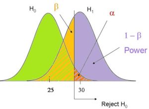
Type I Error: We reject the null hypothesis when it is actually true. The probability of committing this type of error is denoted as α .
Type II Error: We fail to reject the null hypothesis when it is actually false. The probability of committing this type of error is denoted as β .

The Relationship Between Alpha and Beta

Ideally researchers want both the probability of committing a type I error and the probability of committing a type II error to be low.

However, a tradeoff exists between these two probabilities. If we decrease the alpha level, we can decrease the probability of rejecting a null hypothesis when it’s actually true, but this actually increases the beta level – the probability that we fail to reject the null hypothesis when it actually is false.

The Relationship Between Power and Beta

The power of a hypothesis test refers to the probability of detecting an effect or difference when an effect or difference is actually present. In other words, it’s the probability of correctly rejecting a false null hypothesis.

It is calculated as:

Power = 1 – β

In general, researchers want the power of a test to be high so that if some effect or difference does exist, the test is able to detect it.

From the equation above, we can see that the best way to raise the power of a test is to reduce the beta level. And the best way to reduce the beta level is typically to increase the sample size.

The following examples shows how to calculate the beta level of a hypothesis test and demonstrate why increasing the sample size can lower the beta level.

Example 1: Calculate Beta for a Hypothesis Test

Suppose a researcher wants to test if the mean weight of widgets produced at a factory is less than 500 ounces. It is known that the standard deviation of the weights is 24 ounces and the researcher decides to collect a random sample of 40 widgets.

He will perform the following hypothesis at α = 0.05:

H 0 : μ = 500
H A : μ < 500

Now imagine that the mean weight of widgets being produced is actually 490 ounces. In other words, the null hypothesis should be rejected.

We can use the following steps to calculate the beta level – the probability of failing to reject the null hypothesis when it actually should be rejected:

Step 1: Find the non-rejection region.

According to the Critical Z Value Calculator , the left-tailed critical value at α = 0.05 is -1.645 .

Step 2: Find the minimum sample mean we will fail to reject.

The test statistic is calculated as z = ( x – μ) / (s/√ n )

Thus, we can solve this equation for the sample mean:

x = μ – z*(s/√ n )
x = 500 – 1.645*(24/√ 40 )
x = 493.758

Step 3: Find the probability of the minimum sample mean actually occurring.

We can calculate this probability as:

P(Z ≥ (493.758 – 490) / (24/√ 40 ))
P(Z ≥ 0.99)

According to the Normal CDF Calculator , the probability that Z ≥ 0.99 is 0.1611 .

Thus, the beta level for this test is β = 0.1611. This means there is a 16.11% chance of failing to detect the difference if the real mean is 490 ounces.

Example 2: Calculate Beta for a Test with a Larger Sample Size

Now suppose the researcher performs the exact same hypothesis test but instead uses a sample size of n = 100 widgets. We can repeat the same three steps to calculate the beta level for this test:

x = 500 – 1.645*(24/√ 100 )
P(Z ≥ (496.05 – 490) / (24/√ 100 ))
P(Z ≥ 2.52)

According to the Normal CDF Calculator , the probability that Z ≥ 2.52 is 0.0059.

Thus, the beta level for this test is β = 0.0059. This means there is only a .59% chance of failing to detect the difference if the real mean is 490 ounces.

Notice that by simply increasing the sample size from 40 to 100, the researcher was able to reduce the beta level from 0.1611 all the way down to .0059.

Bonus: Use this Type II Error Calculator to automatically calculate the beta level of a test.

Additional Resources

Introduction to Hypothesis Testing How to Write a Null Hypothesis (5 Examples) An Explanation of P-Values and Statistical Significance

Published by Zach

Sciencing_Icons_Science SCIENCE

Sciencing_icons_biology biology, sciencing_icons_cells cells, sciencing_icons_molecular molecular, sciencing_icons_microorganisms microorganisms, sciencing_icons_genetics genetics, sciencing_icons_human body human body, sciencing_icons_ecology ecology, sciencing_icons_chemistry chemistry, sciencing_icons_atomic & molecular structure atomic & molecular structure, sciencing_icons_bonds bonds, sciencing_icons_reactions reactions, sciencing_icons_stoichiometry stoichiometry, sciencing_icons_solutions solutions, sciencing_icons_acids & bases acids & bases, sciencing_icons_thermodynamics thermodynamics, sciencing_icons_organic chemistry organic chemistry, sciencing_icons_physics physics, sciencing_icons_fundamentals-physics fundamentals, sciencing_icons_electronics electronics, sciencing_icons_waves waves, sciencing_icons_energy energy, sciencing_icons_fluid fluid, sciencing_icons_astronomy astronomy, sciencing_icons_geology geology, sciencing_icons_fundamentals-geology fundamentals, sciencing_icons_minerals & rocks minerals & rocks, sciencing_icons_earth scructure earth structure, sciencing_icons_fossils fossils, sciencing_icons_natural disasters natural disasters, sciencing_icons_nature nature, sciencing_icons_ecosystems ecosystems, sciencing_icons_environment environment, sciencing_icons_insects insects, sciencing_icons_plants & mushrooms plants & mushrooms, sciencing_icons_animals animals, sciencing_icons_math math, sciencing_icons_arithmetic arithmetic, sciencing_icons_addition & subtraction addition & subtraction, sciencing_icons_multiplication & division multiplication & division, sciencing_icons_decimals decimals, sciencing_icons_fractions fractions, sciencing_icons_conversions conversions, sciencing_icons_algebra algebra, sciencing_icons_working with units working with units, sciencing_icons_equations & expressions equations & expressions, sciencing_icons_ratios & proportions ratios & proportions, sciencing_icons_inequalities inequalities, sciencing_icons_exponents & logarithms exponents & logarithms, sciencing_icons_factorization factorization, sciencing_icons_functions functions, sciencing_icons_linear equations linear equations, sciencing_icons_graphs graphs, sciencing_icons_quadratics quadratics, sciencing_icons_polynomials polynomials, sciencing_icons_geometry geometry, sciencing_icons_fundamentals-geometry fundamentals, sciencing_icons_cartesian cartesian, sciencing_icons_circles circles, sciencing_icons_solids solids, sciencing_icons_trigonometry trigonometry, sciencing_icons_probability-statistics probability & statistics, sciencing_icons_mean-median-mode mean/median/mode, sciencing_icons_independent-dependent variables independent/dependent variables, sciencing_icons_deviation deviation, sciencing_icons_correlation correlation, sciencing_icons_sampling sampling, sciencing_icons_distributions distributions, sciencing_icons_probability probability, sciencing_icons_calculus calculus, sciencing_icons_differentiation-integration differentiation/integration, sciencing_icons_application application, sciencing_icons_projects projects, sciencing_icons_news news.

Share Tweet Email Print
Home ⋅
Math ⋅
Algebra ⋅
Ratios & Proportions

How to Find the Beta With an Alpha Hypothesis

How to Calculate a P-Value

In all statistical hypothesis tests, there are two especially important statistics -- alpha and beta. These values represent, respectively, the probability of a type I error and the probability of a type II error. A type I error is a false positive, or conclusion that states there is a significant relationship in the data when in fact there is no significant relationship. A type II error is a false negative, or conclusion that states there is no relationship in the data when in fact there is a significant relationship. Usually, beta is difficult to find. However, if you already have an alpha hypothesis, you can use mathematical techniques to calculate beta. These techniques require additional information: an alpha value, a sample size and an effect size. The alpha value comes from your alpha hypothesis; it is the probability of type I error. The sample size is the number of data points in your data set. The effect size is usually estimated from past data.

List the values that are needed in the beta calculation. These values include alpha, the effect size and the sample size. If you do not have past data that states a clear effect size, use the value 0.3 to be conservative. Essentially, the effect size is the strength of the relationship in the data; thus 0.3 is usually taken as it is a “moderate” effect size.

Find the Z-score for the value 1 - alpha/2. This Z-score will be used in the beta calculation. After calculating the numerical value for 1 - alpha/2, look up the Z-score corresponding to that value. This is the Z-score needed to calculate beta.

Calculate the Z-score for the value 1 - beta. Divide the effect size by 2 and take the square root. Multiply this result by the effect size. Subtract the Z-score found in the last step from this value to arrive at the Z-score for the value 1 – beta.

Convert the Z-score to 1 - beta as a number. “Reverse” look up the Z-score for 1 - beta by first looking up the Z-score in the Z-table. Trace this Z-score back to the column (or row) to find a number. This number is equal to 1 - beta.

Subtract the number just found from 1. This result is beta.

Virtually every introduction to statistics textbook has a Z-table in the appendix. If you do not have a Z-table on hand, consult a statistics book from your library.

How to calculate a two-tailed test, how to determine the sample size in a quantitative..., how to calculate cv values, what are the different types of correlations, how to calculate confidence levels, how to make a relative frequency table, how to know if something is significant using spss, how to calculate levered beta, how to calculate standard errors, how to calculate a t-statistic, the effects of a small sample size limitation, how to calculate statistical sample sizes, how to interpret a student's t-test results, how to calculate the percentage of another number, how to report a sample size, how to calculate bias, how to calculate the root mse in anova, how to calculate a confidence interval, how to write a hypothesis for correlation.

“Essentials of Biostatistics”; Lisa Sullivan; 2008
“Statistical Misconceptions”; Schuyler Huck; 2009

About the Author

Having obtained a Master of Science in psychology in East Asia, Damon Verial has been applying his knowledge to related topics since 2010. Having written professionally since 2001, he has been featured in financial publications such as SafeHaven and the McMillian Portfolio. He also runs a financial newsletter at Stock Barometer.

Find Your Next Great Science Fair Project! GO

We Have More Great Sciencing Articles!

How to Determine the Sample Size in a Quantitative Research Study

User Preferences

Content preview.

Arcu felis bibendum ut tristique et egestas quis:

Ut enim ad minim veniam, quis nostrud exercitation ullamco laboris
Duis aute irure dolor in reprehenderit in voluptate
Excepteur sint occaecat cupidatat non proident

Keyboard Shortcuts

25.3 - calculating sample size.

Before we learn how to calculate the sample size that is necessary to achieve a hypothesis test with a certain power, it might behoove us to understand the effect that sample size has on power. Let's investigate by returning to our IQ example.

Example 25-3 Section

Let $X$ denote the IQ of a randomly selected adult American. Assume, a bit unrealistically again, that $X$ is normally distributed with unknown mean $\mu$ and (a strangely known) standard deviation of 16. This time, instead of taking a random sample of $n=16$ students, let's increase the sample size to $n=64$. And, while setting the probability of committing a Type I error to $\alpha=0.05$, test the null hypothesis $H_0:\mu=100$ against the alternative hypothesis that $H_A:\mu>100$.

What is the power of the hypothesis test when $\mu=108$, $\mu=112$, and $\mu=116$?

Setting $\alpha$, the probability of committing a Type I error, to 0.05, implies that we should reject the null hypothesis when the test statistic $Z\ge 1.645$, or equivalently, when the observed sample mean is 103.29 or greater:

$ \bar{x} = \mu + z \left(\dfrac{\sigma}{\sqrt{n}} \right) = 100 +1.645\left(\dfrac{16}{\sqrt{64}} \right) = 103.29$

Therefore, the power function \K(\mu)\), when $\mu>100$ is the true value, is:

$ K(\mu) = P(\bar{X} \ge 103.29 | \mu) = P \left(Z \ge \dfrac{103.29 - \mu}{16 / \sqrt{64}} \right) = 1 - \Phi \left(\dfrac{103.29 - \mu}{2} \right)$

Therefore, the probability of rejecting the null hypothesis at the $\alpha=0.05$ level when $\mu=108$ is 0.9907, as calculated here:

$K(108) = 1 - \Phi \left( \dfrac{103.29-108}{2} \right) = 1- \Phi(-2.355) = 0.9907 $

And, the probability of rejecting the null hypothesis at the $\alpha=0.05$ level when $\mu=112$ is greater than 0.9999, as calculated here:

$ K(112) = 1 - \Phi \left( \dfrac{103.29-112}{2} \right) = 1- \Phi(-4.355) = 0.9999\ldots $

And, the probability of rejecting the null hypothesis at the $\alpha=0.05$ level when $\mu=116$ is greater than 0.999999, as calculated here:

$ K(116) = 1 - \Phi \left( \dfrac{103.29-116}{2} \right) = 1- \Phi(-6.355) = 0.999999... $

In summary, in the various examples throughout this lesson, we have calculated the power of testing $H_0:\mu=100$ against $H_A:\mu>100$ for two sample sizes ( $n=16$ and $n=64$) and for three possible values of the mean ( $\mu=108$, $\mu=112$, and $\mu=116$). Here's a summary of our power calculations:

As you can see, our work suggests that for a given value of the mean $\mu$ under the alternative hypothesis, the larger the sample size $n$, the greater the power $K(\mu)$ . Perhaps there is no better way to see this than graphically by plotting the two power functions simultaneously, one when $n=16$ and the other when $n=64$:

As this plot suggests, if we are interested in increasing our chance of rejecting the null hypothesis when the alternative hypothesis is true, we can do so by increasing our sample size $n$. This benefit is perhaps even greatest for values of the mean that are close to the value of the mean assumed under the null hypothesis. Let's take a look at two examples that illustrate the kind of sample size calculation we can make to ensure our hypothesis test has sufficient power.

Example 25-4 Section

Let $X$ denote the crop yield of corn measured in the number of bushels per acre. Assume (unrealistically) that $X$ is normally distributed with unknown mean $\mu$ and standard deviation $\sigma=6$. An agricultural researcher is working to increase the current average yield from 40 bushels per acre. Therefore, he is interested in testing, at the $\alpha=0.05$ level, the null hypothesis $H_0:\mu=40$ against the alternative hypothesis that $H_A:\mu>40$. Find the sample size $n$ that is necessary to achieve 0.90 power at the alternative $\mu=45$.

As is always the case, we need to start by finding a threshold value $c$, such that if the sample mean is larger than $c$, we'll reject the null hypothesis:

That is, in order for our hypothesis test to be conducted at the $\alpha=0.05$ level, the following statement must hold (using our typical $Z$ transformation):

$c = 40 + 1.645 \left( \dfrac{6}{\sqrt{n}} \right) $ (**)

But, that's not the only condition that $c$ must meet, because $c$ also needs to be defined to ensure that our power is 0.90 or, alternatively, that the probability of a Type II error is 0.10. That would happen if there was a 10% chance that our test statistic fell short of $c$ when $\mu=45$, as the following drawing illustrates in blue:

This illustration suggests that in order for our hypothesis test to have 0.90 power, the following statement must hold (using our usual $Z$ transformation):

$c = 45 - 1.28 \left( \dfrac{6}{\sqrt{n}} \right) $ (**)

Aha! We have two (asterisked (**)) equations and two unknowns! All we need to do is equate the equations, and solve for $n$. Doing so, we get:

$40+1.645\left(\frac{6}{\sqrt{n}}\right)=45-1.28\left(\frac{6}{\sqrt{n}}\right)$ $\Rightarrow 5=(1.645+1.28)\left(\frac{6}{\sqrt{n}}\right), \qquad \Rightarrow 5=\frac{17.55}{\sqrt{n}}, \qquad n=(3.51)^2=12.3201\approx 13$

Now that we know we will set $n=13$, we can solve for our threshold value c :

$ c = 40 + 1.645 \left( \dfrac{6}{\sqrt{13}} \right)=42.737 $

So, in summary, if the agricultural researcher collects data on $n=13$ corn plots, and rejects his null hypothesis $H_0:\mu=40$ if the average crop yield of the 13 plots is greater than 42.737 bushels per acre, he will have a 5% chance of committing a Type I error and a 10% chance of committing a Type II error if the population mean $\mu$ were actually 45 bushels per acre.

Example 25-5 Section

Consider $p$, the true proportion of voters who favor a particular political candidate. A pollster is interested in testing at the $\alpha=0.01$ level, the null hypothesis $H_0:9=0.5$ against the alternative hypothesis that $H_A:p>0.5$. Find the sample size $n$ that is necessary to achieve 0.80 power at the alternative $p=0.55$.

In this case, because we are interested in performing a hypothesis test about a population proportion $p$, we use the $Z$-statistic:

$Z = \dfrac{\hat{p}-p_0}{\sqrt{\frac{p_0(1-p_0)}{n}}} $

Again, we start by finding a threshold value $c$, such that if the observed sample proportion is larger than $c$, we'll reject the null hypothesis:

That is, in order for our hypothesis test to be conducted at the $\alpha=0.01$ level, the following statement must hold:

$c = 0.5 + 2.326 \sqrt{ \dfrac{(0.5)(0.5)}{n}} $ (**)

But, again, that's not the only condition that c must meet, because $c$ also needs to be defined to ensure that our power is 0.80 or, alternatively, that the probability of a Type II error is 0.20. That would happen if there was a 20% chance that our test statistic fell short of $c$ when $p=0.55$, as the following drawing illustrates in blue:

This illustration suggests that in order for our hypothesis test to have 0.80 power, the following statement must hold:

$c = 0.55 - 0.842 \sqrt{ \dfrac{(0.55)(0.45)}{n}} $ (**)

Again, we have two (asterisked (**)) equations and two unknowns! All we need to do is equate the equations, and solve for $n$. Doing so, we get:

$0.5+2.326\sqrt{\dfrac{0.5(0.5)}{n}}=0.55-0.842\sqrt{\dfrac{0.55(0.45)}{n}} \\ 2.326\dfrac{\sqrt{0.25}}{\sqrt{n}}+0.842\dfrac{\sqrt{0.2475}}{\sqrt{n}}=0.55-0.5 \\ \dfrac{1}{\sqrt{n}}(1.5818897)=0.05 \qquad \Rightarrow n\approx \left(\dfrac{1.5818897}{0.05}\right)^2 = 1000.95 \approx 1001 $

Now that we know we will set $n=1001$, we can solve for our threshold value $c$:

$c = 0.5 + 2.326 \sqrt{\dfrac{(0.5)(0.5)}{1001}}= 0.5367 $

So, in summary, if the pollster collects data on $n=1001$ voters, and rejects his null hypothesis $H_0:p=0.5$ if the proportion of sampled voters who favor the political candidate is greater than 0.5367, he will have a 1% chance of committing a Type I error and a 20% chance of committing a Type II error if the population proportion $p$ were actually 0.55.

Incidentally, we can always check our work! Conducting the survey and subsequent hypothesis test as described above, the probability of committing a Type I error is:

$\alpha= P(\hat{p} >0.5367 \text { if } p = 0.50) = P(Z > 2.3257) = 0.01 $

and the probability of committing a Type II error is:

$\beta = P(\hat{p} <0.5367 \text { if } p = 0.55) = P(Z < -0.846) = 0.199 $

just as the pollster had desired.

We've illustrated several sample size calculations. Now, let's summarize the information that goes into a sample size calculation. In order to determine a sample size for a given hypothesis test, you need to specify:

The desired $\alpha$ level, that is, your willingness to commit a Type I error.

The desired power or, equivalently, the desired $\beta$ level, that is, your willingness to commit a Type II error.

A meaningful difference from the value of the parameter that is specified in the null hypothesis.

The standard deviation of the sample statistic or, at least, an estimate of the standard deviation (the "standard error") of the sample statistic.

A Guide on Data Analysis

14 hypothesis testing.

Error types:

Type I Error (False Positive):

Reality: nope
Diagnosis/Analysis: yes

Type II Error (False Negative):

Reality: yes
Diagnosis/Analysis: nope

Power: The probability of rejecting the null hypothesis when it is actually false

Always written in terms of the population parameter ( $\beta$ ) not the estimator/estimate ( $\hat{\beta}$ )

Sometimes, different disciplines prefer to use $\beta$ (i.e., standardized coefficient), or $\mathbf{b}$ (i.e., unstandardized coefficient)

$\beta$ and $\mathbf{b}$ are similar in interpretation; however, $\beta$ is scale free. Hence, you can see the relative contribution of $\beta$ to the dependent variable. On the other hand, $\mathbf{b}$ can be more easily used in policy decisions.

\[ \beta_j = \mathbf{b} \frac{s_{x_j}}{s_y} \]

Assuming the null hypothesis is true, what is the (asymptotic) distribution of the estimator

\[ \begin{aligned} &H_0: \beta_j = 0 \\ &H_1: \beta_j \neq 0 \end{aligned} \]

then under the null, the OLS estimator has the following distribution

\[ A1-A3a, A5: \sqrt{n} \hat{\beta_j} \sim N(0,Avar(\sqrt{n}\hat{\beta}_j)) \]

For the one-sided test, the null is a set of values, so now you choose the worst case single value that is hardest to prove and derive the distribution under the null

\[ \begin{aligned} &H_0: \beta_j\ge 0 \\ &H_1: \beta_j < 0 \end{aligned} \]

then the hardest null value to prove is $H_0: \beta_j=0$ . Then under this specific null, the OLS estimator has the following asymptotic distribution

\[ A1-A3a, A5: \sqrt{n}\hat{\beta_j} \sim N(0,Avar(\sqrt{n}\hat{\beta}_j)) \]

14.1 Types of hypothesis testing

$H_0 : \theta = \theta_0$

$H_1 : \theta \neq \theta_0$

How far away / extreme $\theta$ can be if our null hypothesis is true

Assume that our likelihood function for q is $L(q) = q^{30}(1-q)^{70}$ Likelihood function

Log-Likelihood function

Figure from ( Fox 1997 )

typically, The likelihood ratio test (and Lagrange Multiplier (Score) ) performs better with small to moderate sample sizes, but the Wald test only requires one maximization (under the full model).

14.2 Wald test

\[ \begin{aligned} W &= (\hat{\theta}-\theta_0)'[cov(\hat{\theta})]^{-1}(\hat{\theta}-\theta_0) \\ W &\sim \chi_q^2 \end{aligned} \]

where $cov(\hat{\theta})$ is given by the inverse Fisher Information matrix evaluated at $\hat{\theta}$ and q is the rank of $cov(\hat{\theta})$ , which is the number of non-redundant parameters in $\theta$

Alternatively,

\[ t_W=\frac{(\hat{\theta}-\theta_0)^2}{I(\theta_0)^{-1}} \sim \chi^2_{(v)} \]

where v is the degree of freedom.

Equivalently,

\[ s_W= \frac{\hat{\theta}-\theta_0}{\sqrt{I(\hat{\theta})^{-1}}} \sim Z \]

How far away in the distribution your sample estimate is from the hypothesized population parameter.

For a null value, what is the probability you would have obtained a realization “more extreme” or “worse” than the estimate you actually obtained?

Significance Level ( $\alpha$ ) and Confidence Level ( $1-\alpha$ )

The significance level is the benchmark in which the probability is so low that we would have to reject the null
The confidence level is the probability that sets the bounds on how far away the realization of the estimator would have to be to reject the null.

Test Statistics

Standardized (transform) the estimator and null value to a test statistic that always has the same distribution
Test Statistic for the OLS estimator for a single hypothesis

\[ T = \frac{\sqrt{n}(\hat{\beta}_j-\beta_{j0})}{\sqrt{n}SE(\hat{\beta_j})} \sim^a N(0,1) \]

\[ T = \frac{(\hat{\beta}_j-\beta_{j0})}{SE(\hat{\beta_j})} \sim^a N(0,1) \]

the test statistic is another random variable that is a function of the data and null hypothesis.

T denotes the random variable test statistic
t denotes the single realization of the test statistic

Evaluating Test Statistic: determine whether or not we reject or fail to reject the null hypothesis at a given significance / confidence level

Three equivalent ways

Critical Value

Confidence Interval

For a given significance level, will determine the critical value $(c)$

One-sided: $H_0: \beta_j \ge \beta_{j0}$

\[ P(T<c|H_0)=\alpha \]

Reject the null if $t<c$

One-sided: $H_0: \beta_j \le \beta_{j0}$

\[ P(T>c|H_0)=\alpha \]

Reject the null if $t>c$

Two-sided: $H_0: \beta_j \neq \beta_{j0}$

\[ P(|T|>c|H_0)=\alpha \]

Reject the null if $|t|>c$

Calculate the probability that the test statistic was worse than the realization you have

\[ \text{p-value} = P(T<t|H_0) \]

\[ \text{p-value} = P(T>t|H_0) \]

\[ \text{p-value} = P(|T|<t|H_0) \]

reject the null if p-value $< \alpha$

Using the critical value associated with a null hypothesis and significance level, create an interval

\[ CI(\hat{\beta}_j)_{\alpha} = [\hat{\beta}_j-(c \times SE(\hat{\beta}_j)),\hat{\beta}_j+(c \times SE(\hat{\beta}_j))] \]

If the null set lies outside the interval then we reject the null.

We are not testing whether the true population value is close to the estimate, we are testing that given a field true population value of the parameter, how like it is that we observed this estimate.
Can be interpreted as we believe with $(1-\alpha)\times 100 \%$ probability that the confidence interval captures the true parameter value.

With stronger assumption (A1-A6), we could consider Finite Sample Properties

\[ T = \frac{\hat{\beta}_j-\beta_{j0}}{SE(\hat{\beta}_j)} \sim T(n-k) \]

This above distributional derivation is strongly dependent on A4 and A5
T has a student t-distribution because the numerator is normal and the denominator is $\chi^2$ .
Critical value and p-values will be calculated from the student t-distribution rather than the standard normal distribution.
$n \to \infty$ , $T(n-k)$ is asymptotically standard normal.

Rule of thumb

if $n-k>120$ : the critical values and p-values from the t-distribution are (almost) the same as the critical values and p-values from the standard normal distribution.

if $n-k<120$

if (A1-A6) hold then the t-test is an exact finite distribution test
if (A1-A3a, A5) hold, because the t-distribution is asymptotically normal, computing the critical values from a t-distribution is still a valid asymptotic test (i.e., not quite the right critical values and p0values, the difference goes away as $n \to \infty$ )

14.2.1 Multiple Hypothesis

test multiple parameters as the same time

$H_0: \beta_1 = 0\ \& \ \beta_2 = 0$
$H_0: \beta_1 = 1\ \& \ \beta_2 = 0$

perform a series of simply hypothesis does not answer the question (joint distribution vs. two marginal distributions).

The test statistic is based on a restriction written in matrix form.

\[ y=\beta_0+x_1\beta_1 + x_2\beta_2 + x_3\beta_3 + \epsilon \]

Null hypothesis is $H_0: \beta_1 = 0$ & $\beta_2=0$ can be rewritten as $H_0: \mathbf{R}\beta -\mathbf{q}=0$ where

$\mathbf{R}$ is a $m \times k$ matrix where m is the number of restrictions and $k$ is the number of parameters. $\mathbf{q}$ is a $k \times 1$ vector
$\mathbf{R}$ “picks up” the relevant parameters while $\mathbf{q}$ is a the null value of the parameter

\[ \mathbf{R}= \left( \begin{array}{cccc} 0 & 1 & 0 & 0 \\ 0 & 0 & 1 & 0 \\ \end{array} \right), \mathbf{q} = \left( \begin{array}{c} 0 \\ 0 \\ \end{array} \right) \]

Test Statistic for OLS estimator for a multiple hypothesis

\[ F = \frac{(\mathbf{R\hat{\beta}-q})\hat{\Sigma}^{-1}(\mathbf{R\hat{\beta}-q})}{m} \sim^a F(m,n-k) \]

$\hat{\Sigma}^{-1}$ is the estimator for the asymptotic variance-covariance matrix

if A4 holds, both the homoskedastic and heteroskedastic versions produce valid estimator
If A4 does not hold, only the heteroskedastic version produces valid estimators.

When $m = 1$ , there is only a single restriction, then the $F$ -statistic is the $t$ -statistic squared.

$F$ distribution is strictly positive, check F-Distribution for more details.

14.2.2 Linear Combination

Testing multiple parameters as the same time

\[ \begin{aligned} H_0&: \beta_1 -\beta_2 = 0 \\ H_0&: \beta_1 - \beta_2 > 0 \\ H_0&: \beta_1 - 2\times\beta_2 =0 \end{aligned} \]

Each is a single restriction on a function of the parameters.

Null hypothesis:

\[ H_0: \beta_1 -\beta_2 = 0 \]

can be rewritten as

\[ H_0: \mathbf{R}\beta -\mathbf{q}=0 \]

where $\mathbf{R}$ =(0 1 -1 0 0) and $\mathbf{q}=0$

14.2.3 Estimate Difference in Coefficients

There is no package to estimate for the difference between two coefficients and its CI, but a simple function created by Katherine Zee can be used to calculate this difference. Some modifications might be needed if you don’t use standard lm model in R.

14.2.4 Application

14.2.5 nonlinear.

Suppose that we have q nonlinear functions of the parameters \[ \mathbf{h}(\theta) = \{ h_1 (\theta), ..., h_q (\theta)\}' \]

The,n, the Jacobian matrix ( $\mathbf{H}(\theta)$ ), of rank q is

\[ \mathbf{H}_{q \times p}(\theta) = \left( \begin{array} {ccc} \frac{\partial h_1(\theta)}{\partial \theta_1} & ... & \frac{\partial h_1(\theta)}{\partial \theta_p} \\ . & . & . \\ \frac{\partial h_q(\theta)}{\partial \theta_1} & ... & \frac{\partial h_q(\theta)}{\partial \theta_p} \end{array} \right) \]

where the null hypothesis $H_0: \mathbf{h} (\theta) = 0$ can be tested against the 2-sided alternative with the Wald statistic

\[ W = \frac{\mathbf{h(\hat{\theta})'\{H(\hat{\theta})[F(\hat{\theta})'F(\hat{\theta})]^{-1}H(\hat{\theta})'\}^{-1}h(\hat{\theta})}}{s^2q} \sim F_{q,n-p} \]

14.3 The likelihood ratio test

\[ t_{LR} = 2[l(\hat{\theta})-l(\theta_0)] \sim \chi^2_v \]

Compare the height of the log-likelihood of the sample estimate in relation to the height of log-likelihood of the hypothesized population parameter

This test considers a ratio of two maximizations,

\[ \begin{aligned} L_r &= \text{maximized value of the likelihood under $H_0$ (the reduced model)} \\ L_f &= \text{maximized value of the likelihood under $H_0 \cup H_a$ (the full model)} \end{aligned} \]

Then, the likelihood ratio is:

\[ \Lambda = \frac{L_r}{L_f} \]

which can’t exceed 1 (since $L_f$ is always at least as large as $L-r$ because $L_r$ is the result of a maximization under a restricted set of the parameter values).

The likelihood ratio statistic is:

\[ \begin{aligned} -2ln(\Lambda) &= -2ln(L_r/L_f) = -2(l_r - l_f) \\ \lim_{n \to \infty}(-2ln(\Lambda)) &\sim \chi^2_v \end{aligned} \]

where $v$ is the number of parameters in the full model minus the number of parameters in the reduced model.

If $L_r$ is much smaller than $L_f$ (the likelihood ratio exceeds $\chi_{\alpha,v}^2$ ), then we reject he reduced model and accept the full model at $\alpha \times 100 \%$ significance level

14.4 Lagrange Multiplier (Score)

\[ t_S= \frac{S(\theta_0)^2}{I(\theta_0)} \sim \chi^2_v \]

where $v$ is the degree of freedom.

Compare the slope of the log-likelihood of the sample estimate in relation to the slope of the log-likelihood of the hypothesized population parameter

14.5 Two One-Sided Tests (TOST) Equivalence Testing

This is a good way to test whether your population effect size is within a range of practical interest (e.g., if the effect size is 0).

school Campus Bookshelves
menu_book Bookshelves
perm_media Learning Objects
login Login
how_to_reg Request Instructor Account
hub Instructor Commons
Download Page (PDF)
Download Full Book (PDF)
Periodic Table
Physics Constants
Scientific Calculator
Reference & Cite
Tools expand_more
Readability

selected template will load here

This action is not available.

11.1: Testing the Hypothesis that β = 0

Last updated
Save as PDF
Page ID 26113

The correlation coefficient, $r$, tells us about the strength and direction of the linear relationship between $x$ and $y$. However, the reliability of the linear model also depends on how many observed data points are in the sample. We need to look at both the value of the correlation coefficient $r$ and the sample size $n$, together. We perform a hypothesis test of the "significance of the correlation coefficient" to decide whether the linear relationship in the sample data is strong enough to use to model the relationship in the population.

The sample data are used to compute $r$, the correlation coefficient for the sample. If we had data for the entire population, we could find the population correlation coefficient. But because we have only sample data, we cannot calculate the population correlation coefficient. The sample correlation coefficient, $r$, is our estimate of the unknown population correlation coefficient.

The symbol for the population correlation coefficient is $\rho$, the Greek letter "rho."
$\rho =$ population correlation coefficient (unknown)
$r =$ sample correlation coefficient (known; calculated from sample data)

The hypothesis test lets us decide whether the value of the population correlation coefficient $\rho$ is "close to zero" or "significantly different from zero". We decide this based on the sample correlation coefficient $r$ and the sample size $n$.

If the test concludes that the correlation coefficient is significantly different from zero, we say that the correlation coefficient is "significant."

Conclusion: There is sufficient evidence to conclude that there is a significant linear relationship between $x$ and $y$ because the correlation coefficient is significantly different from zero.
What the conclusion means: There is a significant linear relationship between $x$ and $y$. We can use the regression line to model the linear relationship between $x$ and $y$ in the population.

If the test concludes that the correlation coefficient is not significantly different from zero (it is close to zero), we say that correlation coefficient is "not significant".

Conclusion: "There is insufficient evidence to conclude that there is a significant linear relationship between $x$ and $y$ because the correlation coefficient is not significantly different from zero."
What the conclusion means: There is not a significant linear relationship between $x$ and $y$. Therefore, we CANNOT use the regression line to model a linear relationship between $x$ and $y$ in the population.
If $r$ is significant and the scatter plot shows a linear trend, the line can be used to predict the value of $y$ for values of $x$ that are within the domain of observed $x$ values.
If $r$ is not significant OR if the scatter plot does not show a linear trend, the line should not be used for prediction.
If $r$ is significant and if the scatter plot shows a linear trend, the line may NOT be appropriate or reliable for prediction OUTSIDE the domain of observed $x$ values in the data.

PERFORMING THE HYPOTHESIS TEST

Null Hypothesis: $H_{0}: \rho = 0$
Alternate Hypothesis: $H_{a}: \rho \neq 0$

WHAT THE HYPOTHESES MEAN IN WORDS:

Null Hypothesis $H_{0}$ : The population correlation coefficient IS NOT significantly different from zero. There IS NOT a significant linear relationship(correlation) between $x$ and $y$ in the population.
Alternate Hypothesis $H_{a}$ : The population correlation coefficient IS significantly DIFFERENT FROM zero. There IS A SIGNIFICANT LINEAR RELATIONSHIP (correlation) between $x$ and $y$ in the population.

DRAWING A CONCLUSION:There are two methods of making the decision. The two methods are equivalent and give the same result.

Method 1: Using the $p\text{-value}$
Method 2: Using a table of critical values

In this chapter of this textbook, we will always use a significance level of 5%, $\alpha = 0.05$

Using the $p\text{-value}$ method, you could choose any appropriate significance level you want; you are not limited to using $\alpha = 0.05$. But the table of critical values provided in this textbook assumes that we are using a significance level of 5%, $\alpha = 0.05$. (If we wanted to use a different significance level than 5% with the critical value method, we would need different tables of critical values that are not provided in this textbook.)

METHOD 1: Using a $p\text{-value}$ to make a decision

To calculate the $p\text{-value}$ using LinRegTTEST:

On the LinRegTTEST input screen, on the line prompt for $\beta$ or $\rho$, highlight "$\neq 0$"

The output screen shows the $p\text{-value}$ on the line that reads "$p =$".

(Most computer statistical software can calculate the $p\text{-value}$.)

If the $p\text{-value}$ is less than the significance level ( $\alpha = 0.05$ ):

Decision: Reject the null hypothesis.
Conclusion: "There is sufficient evidence to conclude that there is a significant linear relationship between $x$ and $y$ because the correlation coefficient is significantly different from zero."

If the $p\text{-value}$ is NOT less than the significance level ( $\alpha = 0.05$ )

Decision: DO NOT REJECT the null hypothesis.
Conclusion: "There is insufficient evidence to conclude that there is a significant linear relationship between $x$ and $y$ because the correlation coefficient is NOT significantly different from zero."

Calculation Notes:

You will use technology to calculate the $p\text{-value}$. The following describes the calculations to compute the test statistics and the $p\text{-value}$:
The $p\text{-value}$ is calculated using a $t$-distribution with $n - 2$ degrees of freedom.
The formula for the test statistic is $t = \frac{r\sqrt{n-2}}{\sqrt{1-r^{2}}}$. The value of the test statistic, $t$, is shown in the computer or calculator output along with the $p\text{-value}$. The test statistic $t$ has the same sign as the correlation coefficient $r$.
The $p\text{-value}$ is the combined area in both tails.

An alternative way to calculate the $p\text{-value}$ ( $p$ ) given by LinRegTTest is the command 2*tcdf(abs(t),10^99, n-2) in 2nd DISTR.

THIRD-EXAM vs FINAL-EXAM EXAMPLE: $p\text{-value}$ method

Consider the third exam/final exam example.
The line of best fit is: $\hat{y} = -173.51 + 4.83x$ with $r = 0.6631$ and there are $n = 11$ data points.
Can the regression line be used for prediction? Given a third exam score ( $x$ value), can we use the line to predict the final exam score (predicted $y$ value)?
$H_{0}: \rho = 0$
$H_{a}: \rho \neq 0$
$\alpha = 0.05$
The $p\text{-value}$ is 0.026 (from LinRegTTest on your calculator or from computer software).
The $p\text{-value}$, 0.026, is less than the significance level of $\alpha = 0.05$.
Decision: Reject the Null Hypothesis $H_{0}$
Conclusion: There is sufficient evidence to conclude that there is a significant linear relationship between the third exam score ($x$) and the final exam score ($y$) because the correlation coefficient is significantly different from zero.

Because $r$ is significant and the scatter plot shows a linear trend, the regression line can be used to predict final exam scores.

METHOD 2: Using a table of Critical Values to make a decision

The 95% Critical Values of the Sample Correlation Coefficient Table can be used to give you a good idea of whether the computed value of $r$ is significant or not . Compare $r$ to the appropriate critical value in the table. If $r$ is not between the positive and negative critical values, then the correlation coefficient is significant. If $r$ is significant, then you may want to use the line for prediction.

Example $\PageIndex{1}$

Suppose you computed $r = 0.801$ using $n = 10$ data points. $df = n - 2 = 10 - 2 = 8$. The critical values associated with $df = 8$ are $-0.632$ and $+0.632$. If $r <$ negative critical value or $r >$ positive critical value, then $r$ is significant. Since $r = 0.801$ and $0.801 > 0.632$, $r$ is significant and the line may be used for prediction. If you view this example on a number line, it will help you.

Exercise $\PageIndex{1}$

For a given line of best fit, you computed that $r = 0.6501$ using $n = 12$ data points and the critical value is 0.576. Can the line be used for prediction? Why or why not?

If the scatter plot looks linear then, yes, the line can be used for prediction, because $r >$ the positive critical value.

Example $\PageIndex{2}$

Suppose you computed $r = –0.624$ with 14 data points. $df = 14 – 2 = 12$. The critical values are $-0.532$ and $0.532$. Since $-0.624 < -0.532$, $r$ is significant and the line can be used for prediction

Exercise $\PageIndex{2}$

For a given line of best fit, you compute that $r = 0.5204$ using $n = 9$ data points, and the critical value is $0.666$. Can the line be used for prediction? Why or why not?

No, the line cannot be used for prediction, because $r <$ the positive critical value.

Example $\PageIndex{3}$

Suppose you computed $r = 0.776$ and $n = 6$. $df = 6 - 2 = 4$. The critical values are $-0.811$ and $0.811$. Since $-0.811 < 0.776 < 0.811$, $r$ is not significant, and the line should not be used for prediction.

Exercise $\PageIndex{3}$

For a given line of best fit, you compute that $r = -0.7204$ using $n = 8$ data points, and the critical value is $= 0.707$. Can the line be used for prediction? Why or why not?

Yes, the line can be used for prediction, because $r <$ the negative critical value.

THIRD-EXAM vs FINAL-EXAM EXAMPLE: critical value method

Consider the third exam/final exam example. The line of best fit is: $\hat{y} = -173.51 + 4.83x$ with $r = 0.6631$ and there are $n = 11$ data points. Can the regression line be used for prediction? Given a third-exam score ( $x$ value), can we use the line to predict the final exam score (predicted $y$ value)?

Use the "95% Critical Value" table for $r$ with $df = n - 2 = 11 - 2 = 9$.
The critical values are $-0.602$ and $+0.602$
Since $0.6631 > 0.602$, $r$ is significant.
Conclusion:There is sufficient evidence to conclude that there is a significant linear relationship between the third exam score ($x$) and the final exam score ($y$) because the correlation coefficient is significantly different from zero.

Example $\PageIndex{4}$

Suppose you computed the following correlation coefficients. Using the table at the end of the chapter, determine if $r$ is significant and the line of best fit associated with each r can be used to predict a $y$ value. If it helps, draw a number line.

$r = –0.567$ and the sample size, $n$, is $19$. The $df = n - 2 = 17$. The critical value is $-0.456$. $-0.567 < -0.456$ so $r$ is significant.
$r = 0.708$ and the sample size, $n$, is $9$. The $df = n - 2 = 7$. The critical value is $0.666$. $0.708 > 0.666$ so $r$ is significant.
$r = 0.134$ and the sample size, $n$, is $14$. The $df = 14 - 2 = 12$. The critical value is $0.532$. $0.134$ is between $-0.532$ and $0.532$ so $r$ is not significant.
$r = 0$ and the sample size, $n$, is five. No matter what the $dfs$ are, $r = 0$ is between the two critical values so $r$ is not significant.

Exercise $\PageIndex{4}$

For a given line of best fit, you compute that $r = 0$ using $n = 100$ data points. Can the line be used for prediction? Why or why not?

No, the line cannot be used for prediction no matter what the sample size is.

Assumptions in Testing the Significance of the Correlation Coefficient

Testing the significance of the correlation coefficient requires that certain assumptions about the data are satisfied. The premise of this test is that the data are a sample of observed points taken from a larger population. We have not examined the entire population because it is not possible or feasible to do so. We are examining the sample to draw a conclusion about whether the linear relationship that we see between $x$ and $y$ in the sample data provides strong enough evidence so that we can conclude that there is a linear relationship between $x$ and $y$ in the population.

The regression line equation that we calculate from the sample data gives the best-fit line for our particular sample. We want to use this best-fit line for the sample as an estimate of the best-fit line for the population. Examining the scatter plot and testing the significance of the correlation coefficient helps us determine if it is appropriate to do this.

The assumptions underlying the test of significance are:

There is a linear relationship in the population that models the average value of $y$ for varying values of $x$. In other words, the expected value of $y$ for each particular value lies on a straight line in the population. (We do not know the equation for the line for the population. Our regression line from the sample is our best estimate of this line in the population.)
The $y$ values for any particular $x$ value are normally distributed about the line. This implies that there are more $y$ values scattered closer to the line than are scattered farther away. Assumption (1) implies that these normal distributions are centered on the line: the means of these normal distributions of $y$ values lie on the line.
The standard deviations of the population $y$ values about the line are equal for each value of $x$. In other words, each of these normal distributions of $y$ values has the same shape and spread about the line.
The residual errors are mutually independent (no pattern).
The data are produced from a well-designed, random sample or randomized experiment.

Linear regression is a procedure for fitting a straight line of the form $\hat{y} = a + bx$ to data. The conditions for regression are:

Linear In the population, there is a linear relationship that models the average value of $y$ for different values of $x$.
Independent The residuals are assumed to be independent.
Normal The $y$ values are distributed normally for any value of $x$.
Equal variance The standard deviation of the $y$ values is equal for each $x$ value.
Random The data are produced from a well-designed random sample or randomized experiment.

The slope $b$ and intercept $a$ of the least-squares line estimate the slope $\beta$ and intercept $\alpha$ of the population (true) regression line. To estimate the population standard deviation of $y$, $\sigma$, use the standard deviation of the residuals, $s$. $s = \sqrt{\frac{SEE}{n-2}}$. The variable $\rho$ (rho) is the population correlation coefficient. To test the null hypothesis $H_{0}: \rho =$ hypothesized value , use a linear regression t-test. The most common null hypothesis is $H_{0}: \rho = 0$ which indicates there is no linear relationship between $x$ and $y$ in the population. The TI-83, 83+, 84, 84+ calculator function LinRegTTest can perform this test (STATS TESTS LinRegTTest).

Formula Review

Least Squares Line or Line of Best Fit:

\[\hat{y} = a + bx\]

\[a = y\text{-intercept}\]

\[b = \text{slope}\]

Standard deviation of the residuals:

\[s = \sqrt{\frac{SEE}{n-2}}\]

\[SSE = \text{sum of squared errors}\]

\[n = \text{the number of data points}\]

Hypothesis Testing Calculator

Related: confidence interval calculator, type ii error.

The first step in hypothesis testing is to calculate the test statistic. The formula for the test statistic depends on whether the population standard deviation (σ) is known or unknown. If σ is known, our hypothesis test is known as a z test and we use the z distribution. If σ is unknown, our hypothesis test is known as a t test and we use the t distribution. Use of the t distribution relies on the degrees of freedom, which is equal to the sample size minus one. Furthermore, if the population standard deviation σ is unknown, the sample standard deviation s is used instead. To switch from σ known to σ unknown, click on $\boxed{\sigma}$ and select $\boxed{s}$ in the Hypothesis Testing Calculator.

Next, the test statistic is used to conduct the test using either the p-value approach or critical value approach. The particular steps taken in each approach largely depend on the form of the hypothesis test: lower tail, upper tail or two-tailed. The form can easily be identified by looking at the alternative hypothesis (H a ). If there is a less than sign in the alternative hypothesis then it is a lower tail test, greater than sign is an upper tail test and inequality is a two-tailed test. To switch from a lower tail test to an upper tail or two-tailed test, click on $\boxed{\geq}$ and select $\boxed{\leq}$ or $\boxed{=}$, respectively.

In the p-value approach, the test statistic is used to calculate a p-value. If the test is a lower tail test, the p-value is the probability of getting a value for the test statistic at least as small as the value from the sample. If the test is an upper tail test, the p-value is the probability of getting a value for the test statistic at least as large as the value from the sample. In a two-tailed test, the p-value is the probability of getting a value for the test statistic at least as unlikely as the value from the sample.

To test the hypothesis in the p-value approach, compare the p-value to the level of significance. If the p-value is less than or equal to the level of signifance, reject the null hypothesis. If the p-value is greater than the level of significance, do not reject the null hypothesis. This method remains unchanged regardless of whether it's a lower tail, upper tail or two-tailed test. To change the level of significance, click on $\boxed{.05}$. Note that if the test statistic is given, you can calculate the p-value from the test statistic by clicking on the switch symbol twice.

In the critical value approach, the level of significance ($\alpha$) is used to calculate the critical value. In a lower tail test, the critical value is the value of the test statistic providing an area of $\alpha$ in the lower tail of the sampling distribution of the test statistic. In an upper tail test, the critical value is the value of the test statistic providing an area of $\alpha$ in the upper tail of the sampling distribution of the test statistic. In a two-tailed test, the critical values are the values of the test statistic providing areas of $\alpha / 2$ in the lower and upper tail of the sampling distribution of the test statistic.

To test the hypothesis in the critical value approach, compare the critical value to the test statistic. Unlike the p-value approach, the method we use to decide whether to reject the null hypothesis depends on the form of the hypothesis test. In a lower tail test, if the test statistic is less than or equal to the critical value, reject the null hypothesis. In an upper tail test, if the test statistic is greater than or equal to the critical value, reject the null hypothesis. In a two-tailed test, if the test statistic is less than or equal the lower critical value or greater than or equal to the upper critical value, reject the null hypothesis.

When conducting a hypothesis test, there is always a chance that you come to the wrong conclusion. There are two types of errors you can make: Type I Error and Type II Error. A Type I Error is committed if you reject the null hypothesis when the null hypothesis is true. Ideally, we'd like to accept the null hypothesis when the null hypothesis is true. A Type II Error is committed if you accept the null hypothesis when the alternative hypothesis is true. Ideally, we'd like to reject the null hypothesis when the alternative hypothesis is true.

Hypothesis testing is closely related to the statistical area of confidence intervals. If the hypothesized value of the population mean is outside of the confidence interval, we can reject the null hypothesis. Confidence intervals can be found using the Confidence Interval Calculator . The calculator on this page does hypothesis tests for one population mean. Sometimes we're interest in hypothesis tests about two population means. These can be solved using the Two Population Calculator . The probability of a Type II Error can be calculated by clicking on the link at the bottom of the page.

Statistics Resources

Excel - Tutorials
Basic Probability Rules
Single Event Probability
Complement Rule
Levels of Measurement
Independent and Dependent Variables
Entering Data
Central Tendency
Data and Tests
Displaying Data
Discussing Statistics In-text
SEM and Confidence Intervals
Two-Way Frequency Tables
Empirical Rule
Finding Probability
Accessing SPSS
Chart and Graphs
Frequency Table and Distribution
Descriptive Statistics
Converting Raw Scores to Z-Scores
Converting Z-scores to t-scores
Split File/Split Output
Partial Eta Squared
Downloading and Installing G*Power: Windows/PC
Correlation
Testing Parametric Assumptions
One-Way ANOVA
Two-Way ANOVA
Repeated Measures ANOVA
Goodness-of-Fit
Test of Association
Pearson's r
Point Biserial
Mediation and Moderation
Simple Linear Regression
Multiple Linear Regression
Binomial Logistic Regression
Multinomial Logistic Regression
Independent Samples T-test
Dependent Samples T-test
Testing Assumptions
T-tests using SPSS
T-Test Practice
Predictive Analytics This link opens in a new window
Quantitative Research Questions
Null & Alternative Hypotheses
One-Tail vs. Two-Tail

Alpha & Beta

Associated Probability
Decision Rule
Statement of Conclusion
Statistics Group Sessions

ASC Chat Hours

ASC Chat is usually available at the following times ( Pacific Time):

If there is not a coach on duty, submit your question via one of the below methods:

928-440-1325

Ask a Coach

[email protected]

Search our FAQs on the Academic Success Center's Ask a Coach page.

In hypothesis testing, there are two important values you should be familiar with: alpha (α) and beta (β). These values are used to determine how meaningful the results of the test are. So, let’s talk about them!

Alpha is also known as the level of significance. This represents the probability of obtaining your results due to chance. The smaller this value is, the more “unusual” the results, indicating that the sample is from a different population than it’s being compared to, for example. Commonly, this value is set to .05 (or 5%), but can take on any value chosen by the research not exceeding .05.

Alpha also represents your chance of making a Type I Error . What’s that? The chance that you reject the null hypothesis when in reality, you should fail to reject the null hypothesis. In other words, your sample data indicates that there is a difference when in reality, there is not. Like a false positive.

Multiple Hypothesis Testing

When a study includes more than one hypothesis test, the alpha of the test will not match the alpha for each test. There is a cumulative effect of alpha when multiple tests are being conducted such that three tests using alpha=.05 each would have a cumulative alpha of .15 for the study. This exceeds what is acceptable for quantitative research. Therefore, researchers should consider making an adjustment, such as a Bonferroni Correction . Using this method, the researcher takes the alpha of the study and divides it by the number of tests being conducted: .05/5 = .01. The result is the level of significance that will be used for each test to determine significance.

The other key-value relates to the power of your study. Power refers to your study’s ability to find a difference if there is one. It logically follows that the greater the power, the more meaningful your results are. Beta = 1 – Power. Values of beta should be kept small, but do not have to be as small as alpha values. Values between .05 and .20 are acceptable.

Beta also represents the chance of making a Type II Error . As you may have guessed, this means that you came to the wrong conclusion in your study, but it’s the opposite of a Type I Error. With a Type II Error, you incorrectly fail to reject the null. In simpler terms, the data indicates that there is not a significant difference when in reality there is. Your study failed to capture a significant finding. Like a false negative.

Type I Error: Testing positive for antibodies, when in fact, no antibodies are present. Type II Error: Testing negative for antibodies when in fact, antibodies are present.

Was this resource helpful?

<< Previous: One-Tail vs. Two-Tail
Next: Associated Probability >>
Last Updated: Apr 2, 2024 6:35 PM
URL: https://resources.nu.edu/statsresources

Confusing Statistical Terms #2: Alpha and Beta

by Karen Grace-Martin 28 Comments

Oh so many years ago I had my first insight into just how ridiculously confusing all the statistical terminology can be for novices.

I was TAing a two-semester applied statistics class for graduate students in biology. It started with basic hypothesis testing and went on through to multiple regression.

It was a cross-listed class, meaning there were a handful of courageous (or masochistic) undergrads in the class, and they were having trouble keeping up with the ambitious graduate-level pace.

I remember one day in particular. I was leading a discussion section when one of the poor undergrads was hopelessly lost. We were talking about the simple regression–a regression model with only one predictor variable. She was stuck on understanding the regression coefficient (beta) and the intercept .

In most textbooks, the regression slope coefficient is denoted by β 1 and the intercept is denoted by β 0 . But in the one we were using (and I’ve seen this in others) the regression slope coefficient was denoted by β (beta), and the intercept was denoted by α (alpha). I guess the advantage of this is to not have to include subscripts.

It was only after repeated probing that I realized she was logically trying to fit what we were talking about into the concepts of alpha and beta that we had already taught her–Type I and Type II errors in hypothesis testing.

Entirely. Different. Concepts.

With the same names.

Once I realized the source of the misunderstanding, I was able to explain that we were using the same terminology for entirely different concepts.

But as it turns out, there are even more meanings of both alpha and beta in statistics. Here they all are:

Hypothesis testing

As I already mentioned, the definition most learners of statistics come to first for beta and alpha are about hypothesis testing.

α (Alpha) is the probability of Type I error in any hypothesis test–incorrectly rejecting the null hypothesis.

β (Beta) is the probability of Type II error in any hypothesis test–incorrectly failing to reject the null hypothesis. (1 – β is power).

Population Regression coefficients

In most textbooks and software packages, the population regression coefficients are denoted by β.

Like all population parameters, they are theoretical–we don’t know their true values. The regression coefficients we estimate from our sample are estimates of those parameter values. Most parameters are denoted with Greek letters and statistics with the corresponding Latin letters.

Most texts refer to the intercept as β 0 ( beta-naught ) and every other regression coefficient as β 1 , β 2 , β 3 , etc. But as I already mentioned, some statistics texts will refer to the intercept as α, to distinguish it from the other coefficients.

If the β has a ^ over it, it’s called beta-hat and is the sample estimate of the population parameter β. And to make that even more confusing, sometimes instead of beta-hat, those sample estimates are denoted B or b.

Standardized Regression Coefficient Estimates

But, for some reason, SPSS labels standardized regression coefficient estimates as Beta . Despite the fact that they are statistics–measured on the sample, not the population.

More confusion.

And I can’t verify this, but I vaguely recall that Systat uses the same term. If you have Systat and can verify or negate this claim, feel free to do so in the comments.

Cronbach’s alpha

Another, completely separate use of alpha is Cronbach’s alpha , aka Coefficient Alpha, which measures the reliability of a scale.

It’s a very useful little statistic, but should not be confused with either of the other uses of alpha.

Beta Distribution and Beta Regression

You may have also heard of Beta regression, which is a generalized linear model based on the beta distribution .

The beta distribution is another distribution in statistics, just like the normal, Poisson, or binomial distributions. There are dozens of distributions in statistics, but some are used and taught more than others, so you may not have heard of this one.

The beta distribution has nothing to do with any of the other uses of the term beta.

Other uses of Alpha and Beta

If you really start to get into higher level statistics, you’ll see alpha and beta used quite often as parameters in different distributions. I don’t know if they’re commonly used simply because everyone knows those Greek letters. But you’ll see them, for example, as parameters of a gamma distribution. Relatedly, you’ll see alpha as a parameter of a negative binomial distribution.

If you think of other uses of alpha or beta, please leave them in the comments.

See the full Series on Confusing Statistical Terms .

Reader Interactions

April 26, 2021 at 8:49 am

The first place I think the terminology drives my high school kids crazy is when we no longer write the equation of a line as y = mx + b like in algebra, but write it y = a + bx.

In algebra, b was the y-intercept. Now it’s slope. Geez, why do we do this to kids?

June 9, 2021 at 11:21 am

To be fair, one very important lesson in ones journey through maths is to not stick too much with certain letters for variables. It is always in relation to something. A hard lesson but a worthy one, imo.

June 22, 2021 at 9:53 am

I think it’s because in statistics, we use m for means. I don’t know why all the algebra textbooks use m for a slope, but yes, I get your point.

But I’ve found that pointing it out that this is confusing is really helpful to people who are confused.

June 6, 2020 at 8:06 pm

I really like the Hypothesis Testing graph. It’s one of the most comprehensive I’ve seen. Thank you for posting!

June 30, 2018 at 11:00 am

Thank you this is very helpful. I’m new to genomics and I get confused about alpha and beta when people talk about it. In genomics people use both regression and hypothesis testing frequently so I’m getting more confused and mixing up the betas. Now it’s clear to me after reading this post. Can you please talk about effect size and p-values as well?

January 20, 2017 at 1:04 pm

kindly tell me if alpha+beta what will be answer

April 15, 2017 at 12:53 am

It’s a formulae…apha×beta =-b/a

April 15, 2017 at 12:54 am

Sorry…alpha+beta=-b/a

December 14, 2016 at 3:59 pm

Hi, I am comparing stock returns on a monthly and daily basis, there are differences between the outcomes of the Hypothesis tests. Could you tell me a possible reason/s for the results?

September 14, 2016 at 11:52 am

I have a confussion regarding the name and use of the product of dividing the estimator (coefficient) of a variable by its S.E.. In some places I found the called this Est./S.E. as standardized regression coefficient, is that right? Thanks

February 29, 2016 at 12:27 pm

hey, i was wondering if you can explain to me the assumptions that are needed for a and b to be unbiased estimates of Alpha and Beta. thanks ,

November 17, 2015 at 10:03 pm

Thank you so much! You are very kind for spending your time to help others. Bless you and your family

April 10, 2015 at 11:54 am

hi, i am very new to stats and i am doing a multiple regression analysis in spss and two letters confuse me. The spss comes up with a B letter (capital) but here i see all of you talking about β (greek small letter), and when i listen to youtube videos i hear beta wades, what is their difference? Please help!!!!

January 20, 2017 at 3:32 pm

calli, its beta weight.. its a standarized regression coefficient [slope of a line in a regression equation]. it equals correlation when there is a single predictor.

November 14, 2014 at 3:16 pm

Can you tell me why we use alpha?

July 5, 2013 at 10:51 am

wha is bifference between beta and beta hat and u and ui hat

July 8, 2013 at 2:59 pm

Hi Ayesha, great question. The terms without hats are the population parameters. The terms with hats indicate the sample statistic, which estimates the population parameter.

September 14, 2019 at 2:02 am

but the population parameters are only theoretical, because we can’t get the entire data of nature and society to research? Is that so?

October 28, 2019 at 10:15 am

July 30, 2012 at 1:46 am

Im wondering about the use of “beta 0” In a null hypothesis. What im wanting to test is “The effect of diameter on height = 0, or not equal to 0.

Having a lil trouble remembering the stat101 terminology.

I got the impression that that rather than writing: Ho: Ed on H = 0 Ha: Ed on H ≠ 0 can I use the beta nought symbol like B1 – B2 = 0 etc instead or am I way off track?

August 3, 2012 at 2:57 pm

The effect of diameter on height is most likely the slope, not the intercept. It’s beta1 in this equation:

Height=beta0 + beta1*diameter

Here’s more info about the intercept: https://www.theanalysisfactor.com/interpreting-the-intercept-in-a-regression-model/

September 29, 2011 at 5:16 am

This is so helpful. Thx!!

March 20, 2011 at 4:38 pm

I have read the Type I and Type II distinction about 20 times and still have been confused. I have created mnemonic devices, used visual imagery – the whole nine yards. I just read your description and it clicked. Easy peasy. Thanks!

March 25, 2011 at 12:54 pm

Thanks, Carrie! Glad it was helpful.

February 11, 2011 at 9:54 pm

Hi! This helps, but I am a little confused about this article I am reading. There is a table that lists the variables with Standardized Regression Coefficients. Two of the coefficients have ***. The *** has a note that says “alpha > 0.01”. What is alpha in this case? Is it the intercept? Is this note indicating that these variables are not significant because they are > 0.01? Damn statistics! Why can’t things be less confusing!?!?!

February 18, 2011 at 6:27 pm

Hi Lyndsey,

That’s pretty strange. It’s pretty common to have *** next to coefficients that are significant, i.e. p “, “not p <". And while yes, you want to compare p to alpha, that statement is no equivalent. I'd have to see it to really make sense of it. Can you give us a link?

December 18, 2009 at 8:10 am

I find SPSS’s use of beta for standardised coefficients tremendously annoying!

BTW a beta with a hat on is sometimes used to denote the sample estimate of the population parameter. But mathematicians tend to use any greek letters they feel like using! The trick for maintaining sanity is always to introduce what symbols denote.

December 21, 2009 at 5:38 pm

Ah, yes! Beta hats. This is actually “standard” statistical notation. The sample estimate of any population parameter puts a hat on the parameter. So if beta is the parameter, beta hat is the estimate of that parameter value.

Privacy Overview

What is a Beta Level in Statistics? (Definition & Example)

In statistics, we use hypothesis tests to determine if some assumption about a population parameter is true.

A hypothesis test always has the following two hypotheses:

Null hypothesis (H 0 ): The sample data is consistent with the prevailing belief about the population parameter.

Alternative hypothesis (H A ): The sample data suggests that the assumption made in the null hypothesis is not true. In other words, there is some non-random cause influencing the data.

Whenever we conduct a hypothesis test, there are always four possible outcomes:

There are two types of errors we can commit:

Type I Error: We reject the null hypothesis when it is actually true. The probability of committing this type of error is denoted as α .
Type II Error: We fail to reject the null hypothesis when it is actually false. The probability of committing this type of error is denoted as β .

The Relationship Between Alpha and Beta

Ideally researchers want both the probability of committing a type I error and the probability of committing a type II error to be low.

The Relationship Between Power and Beta

It is calculated as:

Power = 1 – β

In general, researchers want the power of a test to be high so that if some effect or difference does exist, the test is able to detect it.

From the equation above, we can see that the best way to raise the power of a test is to reduce the beta level. And the best way to reduce the beta level is typically to increase the sample size.

The following examples shows how to calculate the beta level of a hypothesis test and demonstrate why increasing the sample size can lower the beta level.

Example 1: Calculate Beta for a Hypothesis Test

He will perform the following hypothesis at α = 0.05:

H 0 : μ = 500

Now imagine that the mean weight of widgets being produced is actually 490 ounces. In other words, the null hypothesis should be rejected.

We can use the following steps to calculate the beta level – the probability of failing to reject the null hypothesis when it actually should be rejected:

Step 1: Find the non-rejection region.

According to the Critical Z Value Calculator , the left-tailed critical value at α = 0.05 is -1.645 .

Step 2: Find the minimum sample mean we will fail to reject.

The test statistic is calculated as z = ( x – μ) / (s/√ n )

Thus, we can solve this equation for the sample mean:

x = μ – z*(s/√ n )
x = 500 – 1.645*(24/√ 40 )
x = 493.758

Step 3: Find the probability of the minimum sample mean actually occurring.

We can calculate this probability as:

P(Z ≥ (493.758 – 490) / (24/√ 40 ))
P(Z ≥ 0.99)

According to the Normal CDF Calculator , the probability that Z ≥ 0.99 is 0.1611 .

Thus, the beta level for this test is β = 0.1611. This means there is a 16.11% chance of failing to detect the difference if the real mean is 490 ounces.

Example 2: Calculate Beta for a Test with a Larger Sample Size

Now suppose the researcher performs the exact same hypothesis test but instead uses a sample size of n = 100 widgets. We can repeat the same three steps to calculate the beta level for this test:

x = 500 – 1.645*(24/√ 100 )
P(Z ≥ (496.05 – 490) / (24/√ 100 ))
P(Z ≥ 2.52)

According to the Normal CDF Calculator , the probability that Z ≥ 2.52 is 0.0059.

Thus, the beta level for this test is β = 0.0059. This means there is only a .59% chance of failing to detect the difference if the real mean is 490 ounces.

Notice that by simply increasing the sample size from 40 to 100, the researcher was able to reduce the beta level from 0.1611 all the way down to .0059.

Bonus: Use this Type II Error Calculator to automatically calculate the beta level of a test.

Additional Resources

Introduction to Hypothesis Testing How to Write a Null Hypothesis (5 Examples) An Explanation of P-Values and Statistical Significance

G-Test of Goodness of Fit Calculator

How to perform a durbin-watson test in excel, related posts, how to normalize data between -1 and 1, vba: how to check if string contains another..., how to interpret f-values in a two-way anova, how to create a vector of ones in..., how to find the mode of a histogram..., how to find quartiles in even and odd..., how to determine if a probability distribution is..., what is a symmetric histogram (definition & examples), how to calculate sxy in statistics (with example), how to calculate sxx in statistics (with example).

Search Search Please fill out this field.
Quantitative Analysis

Beta Risk: What it is, How it Works, Examples

Adam Hayes, Ph.D., CFA, is a financial writer with 15+ years Wall Street experience as a derivatives trader. Besides his extensive derivative trading expertise, Adam is an expert in economics and behavioral finance. Adam received his master's in economics from The New School for Social Research and his Ph.D. from the University of Wisconsin-Madison in sociology. He is a CFA charterholder as well as holding FINRA Series 7, 55 & 63 licenses. He currently researches and teaches economic sociology and the social studies of finance at the Hebrew University in Jerusalem.

Thomas J Catalano is a CFP and Registered Investment Adviser with the state of South Carolina, where he launched his own financial advisory firm in 2018. Thomas' experience gives him expertise in a variety of areas including investments, retirement, insurance, and financial planning.

Katrina Ávila Munichiello is an experienced editor, writer, fact-checker, and proofreader with more than fourteen years of experience working with print and online publications.

What Is Beta Risk?

Beta risk is the probability that a false null hypothesis will be accepted by a statistical test. This is also known as a Type II error or consumer risk. In this context, the term "risk" refers to the chance or likelihood of making an incorrect decision. The primary determinant of the amount of beta risk is the sample size used for the test. Specifically, the larger the sample tested, the lower the beta risk becomes.

Key Takeaways

Beta risk represents the probability that a false hypothesis in a statistical test is accepted as true.
Beta risk contrasts with alpha risk, which measures the probability that a null hypothesis is rejected when it is actually true.
Increasing the sample size used in a statistical test can reduce beta risk.
An acceptable level of beta risk is 10%; beyond that, the sample size should be increased.
Beta, which is part of the capital asset pricing model and measures the relative volatility of a security, is only remotely related to beta risk in decision-making.

Understanding Beta Risk

Beta risk may be defined as the risk found in incorrectly accepting the null hypothesis when an alternative hypothesis is true. Put simply, it is taking the position that there is no difference when, in fact, there is one. A statistical test should be employed to detect differences and the beta risk is the probability that a statistical test will be unable to do so. For example, if beta risk is 0.05, there is a 5% likelihood of inaccuracy.

Beta risk is sometimes called "beta error" and is often paired with " alpha risk ," also known as a Type I error . Alpha risk is an error occurring when a null hypothesis is rejected when it is actually true. It is also known as "producer risk." The best way to decrease alpha risk is to increase the size of the sample being tested with the hope that the larger sample will be more representative of the population.

Beta risk is based on the characteristics and nature of a decision that is being taken and may be determined by a company or individual. It depends on the magnitude of the variance between sample means. The way to manage beta risk is by boosting the test sample size. An acceptable level of beta risk in decision-making is about 10%. Any number higher should trigger increasing the sample size.

Examples of Beta Risk

An interesting application of hypothesis testing in finance can be made using the Altman Z-score. The Z-score is a statistical model meant to predict the future bankruptcy of firms based on certain financial indicators.

Statistical tests of the accuracy of the Z-score have indicated relatively high accuracy, predicting bankruptcy within one year. These tests show a beta risk (firms predicted to go bankrupt but did not) ranging from approximately 15% to 20%, depending on the sample being tested.

In 2007, Altman Z-score indicated that the companies' risks were increasing significantly as the credit ratings of specific asset-related securities had been rated higher than they should have been. The median Altman Z-score of companies in 2007 was 1.81, which is very close to the threshold that would indicate a high probability of becoming bankrupt; Altman's calculations led him to believe a crisis would occur.

The Z-score should be calculated and interpreted with care. For example, the Z-score is not immune to false accounting practices . Since companies in trouble may sometimes misrepresent or cover up their financials, the Z-score is only as accurate as the data that goes into it.

Beta Risk vs. Beta

Beta, in the context of investing, is also known as beta coefficient and is a measure of the volatility, or systematic risk, of a security or a portfolio in comparison to the market as a whole. In short, the beta of an investment indicated whether it is more or less volatile compared to the market.

It is a component of the capital asset pricing model (CAPM), which calculates the expected return of an asset based on its beta and expected market returns. As such, beta is only tangentially related to beta risk in the context of decision-making.

Terms of Service
Editorial Policy
Privacy Policy
Your Privacy Choices

Calculate Beta

A Type II error is defined as not rejecting a false H 0 . The probability of making a Type II error is β, which cannot usually be calculated because one would have to know the true population mean. We calculated β in class, however, to demonstrate its concept and to see what types of things can change the relative size of β.

First Example

Calculating β requires knowing α, n, σ, the H A (and, thus, the H 0 ), and the actual or true population mean. This example, defines these items as:

H A : μ>300
actual population mean is 310

Calculating β is a four-step process. The first step is to identify the null distribution, or the sampling distribution assuming that H 0 is true. In this case, the null distribution is normal (because n=40>30) with a mean of 300 (from assuming that H 0 is true) and a standard ERROR of $\frac{40}{\sqrt{50}}$ =5.657.

The second step is to identify the “rejection wall” on the null distribution. The rejection wall is the sample mean such that values “more extreme” represent rejecting H 0 . In this case, this would be the sample mean that has an area of α “greater” (because H A is a “greater than”). This REVERSE calculation on the null distribution is as follows:

Thus, sample means greater than 307.25 will result in H 0 being rejected, whereas smaller values will lead to H 0 not being rejected. This rejection wall looks like the following on the null distribution.

The third step is to identify the ACTUAL distribution, or the sampling distribution centered on the true population mean. In this case, the actual distribution is also normal (because n=40>30) with a mean of 310 (from the actual population mean given above) and the same standard error of 5.657.

The fourth step is to compute the proportion of sample means in the “do not reject H 0 ” region of the ACTUAL distribution. This FORWARD calculation is shown below and illustrated in the figure below.

Thus, β for this situation is 0.3134.

The second step is always a REVERSE calculation with α more extreme as defined by H A .
The fourth step is always a FORWARD calculation in the OPPOSITE direction of α in the second step.

Second Example

This example, defines these items as:

H A : μ<550
actual population mean is 520

The null distribution in the first step is normal (because n=80>30) with a mean of 550 (from assuming that H 0 is true) and a standard ERROR of $\frac{100}{\sqrt{80}}$ =11.180. The “rejection wall” in the second step is 568.39, which has α “less” (because of H A ).

The actual distributioin in the third step is normal with a mean of 520 and standard error of 11.180. The proportion of sample means in the “do not reject H 0 ” region of the actual distribution for the fourth step is shown below and illustrated in the figure below. Thus, β is 0.1495.

Have a language expert improve your writing

Run a free plagiarism check in 10 minutes, generate accurate citations for free.

Knowledge Base

Hypothesis Testing | A Step-by-Step Guide with Easy Examples

Published on November 8, 2019 by Rebecca Bevans . Revised on June 22, 2023.

Hypothesis testing is a formal procedure for investigating our ideas about the world using statistics . It is most often used by scientists to test specific predictions, called hypotheses, that arise from theories.

There are 5 main steps in hypothesis testing:

State your research hypothesis as a null hypothesis and alternate hypothesis (H o ) and (H a or H 1 ).
Collect data in a way designed to test the hypothesis.
Perform an appropriate statistical test .
Decide whether to reject or fail to reject your null hypothesis.
Present the findings in your results and discussion section.

Though the specific details might vary, the procedure you will use when testing a hypothesis will always follow some version of these steps.

Step 1: state your null and alternate hypothesis, step 2: collect data, step 3: perform a statistical test, step 4: decide whether to reject or fail to reject your null hypothesis, step 5: present your findings, other interesting articles, frequently asked questions about hypothesis testing.

After developing your initial research hypothesis (the prediction that you want to investigate), it is important to restate it as a null (H o ) and alternate (H a ) hypothesis so that you can test it mathematically.

The alternate hypothesis is usually your initial hypothesis that predicts a relationship between variables. The null hypothesis is a prediction of no relationship between the variables you are interested in.

H 0 : Men are, on average, not taller than women. H a : Men are, on average, taller than women.

Prevent plagiarism. Run a free check.

For a statistical test to be valid , it is important to perform sampling and collect data in a way that is designed to test your hypothesis. If your data are not representative, then you cannot make statistical inferences about the population you are interested in.

There are a variety of statistical tests available, but they are all based on the comparison of within-group variance (how spread out the data is within a category) versus between-group variance (how different the categories are from one another).

If the between-group variance is large enough that there is little or no overlap between groups, then your statistical test will reflect that by showing a low p -value . This means it is unlikely that the differences between these groups came about by chance.

Alternatively, if there is high within-group variance and low between-group variance, then your statistical test will reflect that with a high p -value. This means it is likely that any difference you measure between groups is due to chance.

Your choice of statistical test will be based on the type of variables and the level of measurement of your collected data .

an estimate of the difference in average height between the two groups.
a p -value showing how likely you are to see this difference if the null hypothesis of no difference is true.

Based on the outcome of your statistical test, you will have to decide whether to reject or fail to reject your null hypothesis.

In most cases you will use the p -value generated by your statistical test to guide your decision. And in most cases, your predetermined level of significance for rejecting the null hypothesis will be 0.05 – that is, when there is a less than 5% chance that you would see these results if the null hypothesis were true.

In some cases, researchers choose a more conservative level of significance, such as 0.01 (1%). This minimizes the risk of incorrectly rejecting the null hypothesis ( Type I error ).

Here's why students love Scribbr's proofreading services

Discover proofreading & editing

The results of hypothesis testing will be presented in the results and discussion sections of your research paper , dissertation or thesis .

In the results section you should give a brief summary of the data and a summary of the results of your statistical test (for example, the estimated difference between group means and associated p -value). In the discussion , you can discuss whether your initial hypothesis was supported by your results or not.

In the formal language of hypothesis testing, we talk about rejecting or failing to reject the null hypothesis. You will probably be asked to do this in your statistics assignments.

However, when presenting research results in academic papers we rarely talk this way. Instead, we go back to our alternate hypothesis (in this case, the hypothesis that men are on average taller than women) and state whether the result of our test did or did not support the alternate hypothesis.

If your null hypothesis was rejected, this result is interpreted as “supported the alternate hypothesis.”

These are superficial differences; you can see that they mean the same thing.

You might notice that we don’t say that we reject or fail to reject the alternate hypothesis . This is because hypothesis testing is not designed to prove or disprove anything. It is only designed to test whether a pattern we measure could have arisen spuriously, or by chance.

If we reject the null hypothesis based on our research (i.e., we find that it is unlikely that the pattern arose by chance), then we can say our test lends support to our hypothesis . But if the pattern does not pass our decision rule, meaning that it could have arisen by chance, then we say the test is inconsistent with our hypothesis .

If you want to know more about statistics , methodology , or research bias , make sure to check out some of our other articles with explanations and examples.

Normal distribution
Descriptive statistics
Measures of central tendency
Correlation coefficient

Methodology

Cluster sampling
Stratified sampling
Types of interviews
Cohort study
Thematic analysis

Research bias

Implicit bias
Cognitive bias
Survivorship bias
Availability heuristic
Nonresponse bias
Regression to the mean

Hypothesis testing is a formal procedure for investigating our ideas about the world using statistics. It is used by scientists to test specific predictions, called hypotheses , by calculating how likely it is that a pattern or relationship between variables could have arisen by chance.

A hypothesis states your predictions about what your research will find. It is a tentative answer to your research question that has not yet been tested. For some research projects, you might have to write several hypotheses that address different aspects of your research question.

A hypothesis is not just a guess — it should be based on existing theories and knowledge. It also has to be testable, which means you can support or refute it through scientific research methods (such as experiments, observations and statistical analysis of data).

Null and alternative hypotheses are used in statistical hypothesis testing . The null hypothesis of a test always predicts no effect or no relationship between variables, while the alternative hypothesis states your research prediction of an effect or relationship.

Cite this Scribbr article

If you want to cite this source, you can copy and paste the citation or click the “Cite this Scribbr article” button to automatically add the citation to our free Citation Generator.

Bevans, R. (2023, June 22). Hypothesis Testing | A Step-by-Step Guide with Easy Examples. Scribbr. Retrieved April 10, 2024, from https://www.scribbr.com/statistics/hypothesis-testing/

Is this article helpful?

Rebecca Bevans

Other students also liked, choosing the right statistical test | types & examples, understanding p values | definition and examples, what is your plagiarism score.

IMAGES

How To Calculate Beta Hypothesis Testing
Beta and the Power of a Hypothesis Test
¿Qué es un nivel beta en estadísticas? (Definición y ejemplo) en 2023 →
How to Calculate Beta
Hypothesis testing tutorial using p value method
Hypothesis Testing Formula

VIDEO

Hypothesis testing with populations part 1
Hypothesis testing with populations part 2
TWO SAMPLE HYPOTHESIS TESTING IN SPSS
hypothesis testing of comparing means of two independent samples
Two-Sample Hypothesis Tests
problems on testing of hypothesis 3

COMMENTS

What is a Beta Level in Statistics? (Definition & Example)
The following examples shows how to calculate the beta level of a hypothesis test and demonstrate why increasing the sample size can lower the beta level. Example 1: Calculate Beta for a Hypothesis Test. Suppose a researcher wants to test if the mean weight of widgets produced at a factory is less than 500 ounces.
5.4.3
Hypothesis testing is a very powerful statistical tool. Next, we will move onto situations where we compare more than one population parameter. Book traversal links for 5.4.3 - The Relationship Between Power, $\beta$, and $\alpha$
How to Find the Beta With an Alpha Hypothesis
This is the Z-score needed to calculate beta. Calculate the Z-score for the value 1 - beta. Divide the effect size by 2 and take the square root. Multiply this result by the effect size. Subtract the Z-score found in the last step from this value to arrive at the Z-score for the value 1 - beta. Convert the Z-score to 1 - beta as a number.
Understanding Alpha, Beta, and Statistical Power
Maybe we need to be 99% sure. The confidence level will depend on your test and how serious the consequences would be if you were wrong. Generally, the standard starting confidence level value is 95% (.95). The alpha value is expressed as 1-CL. If the confidence level was .95 then the alpha value would be .05 or 5%.
PDF Example of Calculating Beta
Thus we have a 74.22% chance of accepting a false null hypothesis. The power of the test is 1-0.7422 = 0.2578 This would mean we have a 25.78% chance of rejecting a false null hypothesis. Title: Microsoft Word - Example of Calculating Beta.docx Author: mlesperance Created Date:
Type I & Type II Errors
Example: Null and alternative hypothesis. You test whether a new drug intervention can alleviate symptoms of an autoimmune disease. In this case: The null hypothesis (H 0) is that the new drug has no effect on symptoms of the disease. The alternative hypothesis (H 1) is that the drug is effective for alleviating symptoms of the disease.
25.3
Before we learn how to calculate the sample size that is necessary to achieve a hypothesis test with a certain power, it might behoove us to understand the effect that sample size has on power. ... (\beta = P(\hat{p} <0.5367 \text { if } p = 0.55) = P(Z < -0.846) = 0.199 \)
Chapter 14 Hypothesis Testing
The test statistic is based on a restriction written in matrix form. y = β0 + x1β1 + x2β2 + x3β3 + ϵ. Null hypothesis is H0: β1 = 0 & β2 = 0 can be rewritten as H0: Rβ − q = 0 where. R is a m × k matrix where m is the number of restrictions and k is the number of parameters. q is a k × 1 vector.
11.1: Testing the Hypothesis that β = 0
11.1: Testing the Hypothesis that β = 0. The correlation coefficient, \ (r\), tells us about the strength and direction of the linear relationship between \ (x\) and \ (y\). However, the reliability of the linear model also depends on how many observed data points are in the sample.
Hypothesis Testing Calculator with Steps
Hypothesis Testing Calculator. The first step in hypothesis testing is to calculate the test statistic. The formula for the test statistic depends on whether the population standard deviation (σ) is known or unknown. If σ is known, our hypothesis test is known as a z test and we use the z distribution. If σ is unknown, our hypothesis test is ...
Hypothesis testing: Calculate beta without PDF of H1
1. The power of a hypothesis test (beta) is a function of effect size (and SEM, and sample size, and test 'size' (alpha). Therefore to calculate power you need to choose values for all of those variables. The choices can be thoughtful (e.g. use estimates from preliminary experimentation) or arbitrary (e.g. use alpha=0.05 just because).
Alpha & Beta
In hypothesis testing, there are two important values you should be familiar with: alpha (α) and beta (β). These values are used to determine how meaningful the results of the test are. So, let's talk about them! Alpha. Alpha is also known as the level of significance. This represents the probability of obtaining your results due to chance.
PDF 5 ALPHA, BETA, AND POWER HYPOTHESIS TESTING
Hypothesis Testing 79 INSTRUCTIONS A. Set up and sample two model populations. 1. Open a new spreadsheet and set up column head-ings as shown in Figure 1. Generate the α symbol by typing an "a." Select the letter in the formula bar and change the font to symbol font. 2. Enter the values shown in cells B5-C6. 3. In cell B7, calculate the
Confusing Statistical Terms #2: Alpha and Beta
Im wondering about the use of "beta 0" In a null hypothesis. What im wanting to test is "The effect of diameter on height = 0, or not equal to 0. Having a lil trouble remembering the stat101 terminology. I got the impression that that rather than writing: Ho: Ed on H = 0 Ha: Ed on H ≠ 0 can I use the beta nought symbol like
PDF Calculating the Risk of Type II Error (beta risk)
To calculate -risk, we need to have: 1. a null-hypothesis value k 2. the form (>;<;6=) of the alternative hypothesis 3. A speci c value of , the level of signi cance for the test. 4. An assumed population standard deviation ˙so we can work with Z Procedure: 1. Based on the test, nd the rejection criterion (\Reject H
What is a Beta Level in Statistics? (Definition & Example)
Thus, the beta level for this test is β = 0.1611. This means there is a 16.11% chance of failing to detect the difference if the real mean is 490 ounces. Example 2: Calculate Beta for a Test with a Larger Sample Size. Now suppose the researcher performs the exact same hypothesis test but instead uses a sample size of n = 100 widgets.
Beta Risk: What it is, How it Works, Examples
Beta risk is the probability that a false null hypothesis will be accepted by a statistical test. This is also known as a Type II error . The primary determinant of ...
Calculate Beta
Calculating β is a four-step process. The first step is to identify the null distribution, or the sampling distribution assuming that H 0 is true. In this case, the null distribution is normal (because n=40>30) with a mean of 300 (from assuming that H 0 is true) and a standard ERROR of 40 50√ 40 50 =5.657. The second step is to identify the ...
Hypothesis Testing
Present the findings in your results and discussion section. Though the specific details might vary, the procedure you will use when testing a hypothesis will always follow some version of these steps. Table of contents. Step 1: State your null and alternate hypothesis. Step 2: Collect data. Step 3: Perform a statistical test.
hypothesis testing
Thanks for contributing an answer to Cross Validated! Please be sure to answer the question.Provide details and share your research! But avoid …. Asking for help, clarification, or responding to other answers.
self study
$\newcommand{\szdp}[1]{\!\left(#1\right)}$ Background Question: A manufacturer claimed that at least $20\%$ of the public preferred his product. A sample of $100$ persons is taken to check his claim. With $\alpha=0.05,$ how small would the sample percentage have to be before the claim could legitimately be refuted? (Notice that this would involve a one-tailed test of the hypothesis.)
hypothesis testing
To calculate this value, you can first acquire under H1 the percentile of the CI upperbound and the percentile of the CI lowerbound, and then take a difference, which is exactly what this piece of code is doing: > mu = 15.1 # assumed actual mean. > p = pt ( (q - mu)/SE, df=n-1); p. 0.097445 0.995168. > diff (p) # p -p.

What is a Beta Level in Statistics? (Definition & Example)

The Relationship Between Alpha and Beta

The Relationship Between Power and Beta

Example 1: Calculate Beta for a Hypothesis Test

Example 2: Calculate Beta for a Test with a Larger Sample Size

Additional Resources

Published by Zach

Sciencing_Icons_Science SCIENCE

How to Find the Beta With an Alpha Hypothesis

How to Calculate a P-Value

Related Articles

Find Your Next Great Science Fair Project! GO

How to Determine the Sample Size in a Quantitative Research Study

User Preferences

Keyboard Shortcuts

Example 25-3 Section

Example 25-4 Section

Example 25-5 Section

A Guide on Data Analysis

14.1 Types of hypothesis testing

14.2 Wald test

14.2.1 Multiple Hypothesis

14.2.2 Linear Combination

14.2.3 Estimate Difference in Coefficients

14.2.4 Application

14.3 The likelihood ratio test

14.4 Lagrange Multiplier (Score)

14.5 Two One-Sided Tests (TOST) Equivalence Testing

11.1: Testing the Hypothesis that β = 0

PERFORMING THE HYPOTHESIS TEST

METHOD 1: Using a \(p\text{-value}\) to make a decision

METHOD 2: Using a table of Critical Values to make a decision

THIRD-EXAM vs FINAL-EXAM EXAMPLE: critical value method

Assumptions in Testing the Significance of the Correlation Coefficient

Formula Review

Hypothesis Testing Calculator

Statistics Resources

Alpha & Beta

ASC Chat Hours

Was this resource helpful?

Confusing Statistical Terms #2: Alpha and Beta

Hypothesis testing

Population Regression coefficients

Standardized Regression Coefficient Estimates

Cronbach’s alpha

Beta Distribution and Beta Regression

Other uses of Alpha and Beta

Reader Interactions

Leave a Reply Cancel reply

Privacy Overview

What is a Beta Level in Statistics? (Definition & Example)

The Relationship Between Alpha and Beta

The Relationship Between Power and Beta

Example 1: Calculate Beta for a Hypothesis Test

Example 2: Calculate Beta for a Test with a Larger Sample Size

Additional Resources

G-Test of Goodness of Fit Calculator

Beta Risk: What it is, How it Works, Examples

What Is Beta Risk?

Key Takeaways

Understanding Beta Risk

Examples of Beta Risk

Beta Risk vs. Beta

Calculate Beta

First Example

Second Example

Have a language expert improve your writing

Hypothesis Testing | A Step-by-Step Guide with Easy Examples

Table of contents

Prevent plagiarism. Run a free check.

Here's why students love Scribbr's proofreading services

Cite this Scribbr article

Is this article helpful?

Rebecca Bevans

IMAGES

VIDEO

COMMENTS