hypothesis testing in biology

1 Hypothesis Testing

Biology is a science, but what exactly is science? What does the study of biology share with other scientific disciplines?  Science  (from the Latin scientia, meaning “knowledge”) can be defined as knowledge about the natural world.

Biologists study the living world by posing questions about it and seeking science-based responses. This approach is common to other sciences as well and is often referred to as the scientific method . The scientific process was used even in ancient times, but it was first documented by England’s Sir Francis Bacon (1561–1626) ( Figure 1 ), who set up inductive methods for scientific inquiry. The scientific method is not exclusively used by biologists but can be applied to almost anything as a logical problem solving method.

The scientific process typically starts with an observation  (often a problem to be solved) that leads to a question.  Science is very good at answering questions having to do with observations about the natural world, but is very bad at answering questions having to do with purely moral questions, aesthetic questions, personal opinions, or what can be generally categorized as spiritual questions. Science has cannot investigate these areas because they are outside the realm of material phenomena, the phenomena of matter and energy, and cannot be observed and measured.

Let’s think about a simple problem that starts with an observation and apply the scientific method to solve the problem. Imagine that one morning when you wake up and flip a the switch to turn on your bedside lamp, the light won’t turn on. That is an observation that also describes a problem: the lights won’t turn on. Of course, you would next ask the question: “Why won’t the light turn on?”

A hypothesis  is a suggested explanation that can be tested. A hypothesis is NOT the question you are trying to answer – it is what you think the answer to the question will be and why .  Several hypotheses may be proposed as answers to one question. For example, one hypothesis about the question “Why won’t the light turn on?” is “The light won’t turn on because the bulb is burned out.” There are also other possible answers to the question, and therefore other hypotheses may be proposed. A second hypothesis is “The light won’t turn on because the lamp is unplugged” or “The light won’t turn on because the power is out.” A hypothesis should be based on credible background information. A hypothesis is NOT just a guess (not even an educated one), although it can be based on your prior experience (such as in the example where the light won’t turn on). In general, hypotheses in biology should be based on a credible, referenced source of information.

A hypothesis must be testable to ensure that it is valid. For example, a hypothesis that depends on what a dog thinks is not testable, because we can’t tell what a dog thinks. It should also be  falsifiable,  meaning that it can be disproven by experimental results. An example of an unfalsifiable hypothesis is “Red is a better color than blue.” There is no experiment that might show this statement to be false. To test a hypothesis, a researcher will conduct one or more experiments designed to eliminate one or more of the hypotheses. This is important: a hypothesis can be disproven, or eliminated, but it can never be proven.  If an experiment fails to disprove a hypothesis, then that explanation (the hypothesis) is supported as the answer to the question. However, that doesn’t mean that later on, we won’t find a better explanation or design a better experiment that will disprove the first hypothesis and lead to a better one.

A variable is any part of the experiment that can vary or change during the experiment. Typically, an experiment only tests one variable and all the other conditions in the experiment are held constant.

• The variable that is being changed or tested is known as the  independent variable .
• The  dependent variable  is the thing (or things) that you are measuring as the outcome of your experiment.
• A  constant  is a condition that is the same between all of the tested groups.
• A confounding variable  is a condition that is not held constant that could affect the experimental results.

Let’s start with the first hypothesis given above for the light bulb experiment: the bulb is burned out. When testing this hypothesis, the independent variable (the thing that you are testing) would be changing the light bulb and the dependent variable is whether or not the light turns on.

• HINT: You should be able to put your identified independent and dependent variables into the phrase “dependent depends on independent”. If you say “whether or not the light turns on depends on changing the light bulb” this makes sense and describes this experiment. In contrast, if you say “changing the light bulb depends on whether or not the light turns on” it doesn’t make sense.

It would be important to hold all the other aspects of the environment constant, for example not messing with the lamp cord or trying to turn the lamp on using a different light switch. If the entire house had lost power during the experiment because a car hit the power pole, that would be a confounding variable.

You may have learned that a hypothesis can be phrased as an “If..then…” statement. Simple hypotheses can be phrased that way (but they must always also include a “because”), but more complicated hypotheses may require several sentences. It is also very easy to get confused by trying to put your hypothesis into this format. Don’t worry about phrasing hypotheses as “if…then” statements – that is almost never done in experiments outside a classroom.

The results  of your experiment are the data that you collect as the outcome.  In the light experiment, your results are either that the light turns on or the light doesn’t turn on. Based on your results, you can make a conclusion. Your conclusion  uses the results to answer your original question.

We can put the experiment with the light that won’t go in into the figure above:

• Observation: the light won’t turn on.
• Question: why won’t the light turn on?
• Hypothesis: the lightbulb is burned out.
• Prediction: if I change the lightbulb (independent variable), then the light will turn on (dependent variable).
• Experiment: change the lightbulb while leaving all other variables the same.
• Analyze the results: the light didn’t turn on.
• Conclusion: The lightbulb isn’t burned out. The results do not support the hypothesis, time to develop a new one!
• Hypothesis 2: the lamp is unplugged.
• Prediction 2: if I plug in the lamp, then the light will turn on.
• Experiment: plug in the lamp
• Analyze the results: the light turned on!
• Conclusion: The light wouldn’t turn on because the lamp was unplugged. The results support the hypothesis, it’s time to move on to the next experiment!

In practice, the scientific method is not as rigid and structured as it might at first appear. Sometimes an experiment leads to conclusions that favor a change in approach; often, an experiment brings entirely new scientific questions to the puzzle. Many times, science does not operate in a linear fashion; instead, scientists continually draw inferences and make generalizations, finding patterns as their research proceeds. Scientific reasoning is more complex than the scientific method alone suggests.

Control Groups

Another important aspect of designing an experiment is the presence of one or more control groups. A control group  allows you to make a comparison that is important for interpreting your results. Control groups are samples that help you to determine that differences between your experimental groups are due to your treatment rather than a different variable – they eliminate alternate explanations for your results (including experimental error and experimenter bias). They increase reliability, often through the comparison of control measurements and measurements of the experimental groups. Often, the control group is a sample that is not treated with the independent variable, but is otherwise treated the same way as your experimental sample. This type of control group is treated the same way as the experimental group except it does not get treated with the independent variable. Therefore, if the results of the experimental group differ from the control group, the difference must be due to the change of the independent, rather than some outside factor. It is common in complex experiments (such as those published in scientific journals) to have more control groups than experimental groups.

Question: Which fertilizer will produce the greatest number of tomatoes when applied to the plants?

Hypothesis : If I apply different brands of fertilizer to tomato plants, the most tomatoes will be produced from plants watered with Brand A because Brand A advertises that it produces twice as many tomatoes as other leading brands.

Experiment:  Purchase 10 tomato plants of the same type from the same nursery. Pick plants that are similar in size and age. Divide the plants into two groups of 5. Apply Brand A to the first group and Brand B to the second group according to the instructions on the packages. After 10 weeks, count the number of tomatoes on each plant.

Independent Variable:  Brand of fertilizer.

Dependent Variable : Number of tomatoes.

• The number of tomatoes produced depends on the brand of fertilizer applied to the plants.

Constants:  amount of water, type of soil, size of pot, amount of light, type of tomato plant, length of time plants were grown.

Confounding variables : any of the above that are not held constant, plant health, diseases present in the soil or plant before it was purchased.

Results:  Tomatoes fertilized with Brand A  produced an average of 20 tomatoes per plant, while tomatoes fertilized with Brand B produced an average of 10 tomatoes per plant.

You’d want to use Brand A next time you grow tomatoes, right? But what if I told you that plants grown without fertilizer produced an average of 30 tomatoes per plant! Now what will you use on your tomatoes?

Results including control group : Tomatoes which received no fertilizer produced more tomatoes than either brand of fertilizer.

Conclusion:  Although Brand A fertilizer produced more tomatoes than Brand B, neither fertilizer should be used because plants grown without fertilizer produced the most tomatoes!

More examples of control groups:

• You observe growth . Does this mean that your spinach is really contaminated? Consider an alternate explanation for growth: the swab, the water, or the plate is contaminated with bacteria. You could use a control group to determine which explanation is true. If you wet one of the swabs and wiped on a nutrient plate, do bacteria grow?
• You don’t observe growth.  Does this mean that your spinach is really safe? Consider an alternate explanation for no growth: Salmonella isn’t able to grow on the type of nutrient you used in your plates. You could use a control group to determine which explanation is true. If you wipe a known sample of Salmonella bacteria on the plate, do bacteria grow?
• You see a reduction in disease symptoms: you might expect a reduction in disease symptoms purely because the person knows they are taking a drug so they believe should be getting better. If the group treated with the real drug does not show more a reduction in disease symptoms than the placebo group, the drug doesn’t really work. The placebo group sets a baseline against which the experimental group (treated with the drug) can be compared.
• You don’t see a reduction in disease symptoms: your drug doesn’t work. You don’t need an additional control group for comparison.
• You would want a “placebo feeder”. This would be the same type of feeder, but with no food in it. Birds might visit a feeder just because they are interested in it; an empty feeder would give a baseline level for bird visits.
• You would want a control group where you knew the enzyme would function. This would be a tube where you did not change the pH. You need this control group so you know your enzyme is working: if you didn’t see a reaction in any of the tubes with the pH adjusted, you wouldn’t know if it was because the enzyme wasn’t working at all or because the enzyme just didn’t work at any of your tested pH values.
• You would also want a control group where you knew the enzyme would not function (no enzyme added). You need the negative control group so you can ensure that there is no reaction taking place in the absence of enzyme: if the reaction proceeds without the enzyme, your results are meaningless.

Text adapted from: OpenStax , Biology. OpenStax CNX. May 27, 2016  http://cnx.org/contents/[email protected]:RD6ERYiU@5/The-Process-of-Science .

MHCC Biology 112: Biology for Health Professions Copyright © 2019 by Lisa Bartee is licensed under a Creative Commons Attribution 4.0 International License , except where otherwise noted.

Share This Book

• school Campus Bookshelves
• menu_book Bookshelves
• perm_media Learning Objects
• login Login
• how_to_reg Request Instructor Account
• hub Instructor Commons
• Download Page (PDF)
• Download Full Book (PDF)
• Periodic Table
• Physics Constants
• Scientific Calculator
• Reference & Cite
• Tools expand_more
• Readability

selected template will load here

This action is not available.

1.4: Basic Concepts of Hypothesis Testing

• Last updated
• Save as PDF
• Page ID 1715

• John H. McDonald
• University of Delaware

Learning Objectives

• One of the main goals of statistical hypothesis testing is to estimate the \(P\) value, which is the probability of obtaining the observed results, or something more extreme, if the null hypothesis were true. If the observed results are unlikely under the null hypothesis, reject the null hypothesis.
• Alternatives to this "frequentist" approach to statistics include Bayesian statistics and estimation of effect sizes and confidence intervals.

Introduction

There are different ways of doing statistics. The technique used by the vast majority of biologists, and the technique that most of this handbook describes, is sometimes called "frequentist" or "classical" statistics. It involves testing a null hypothesis by comparing the data you observe in your experiment with the predictions of a null hypothesis. You estimate what the probability would be of obtaining the observed results, or something more extreme, if the null hypothesis were true. If this estimated probability (the \(P\) value) is small enough (below the significance value), then you conclude that it is unlikely that the null hypothesis is true; you reject the null hypothesis and accept an alternative hypothesis.

Many statisticians harshly criticize frequentist statistics, but their criticisms haven't had much effect on the way most biologists do statistics. Here I will outline some of the key concepts used in frequentist statistics, then briefly describe some of the alternatives.

Null Hypothesis

The null hypothesis is a statement that you want to test. In general, the null hypothesis is that things are the same as each other, or the same as a theoretical expectation. For example, if you measure the size of the feet of male and female chickens, the null hypothesis could be that the average foot size in male chickens is the same as the average foot size in female chickens. If you count the number of male and female chickens born to a set of hens, the null hypothesis could be that the ratio of males to females is equal to a theoretical expectation of a \(1:1\) ratio.

The alternative hypothesis is that things are different from each other, or different from a theoretical expectation.

For example, one alternative hypothesis would be that male chickens have a different average foot size than female chickens; another would be that the sex ratio is different from \(1:1\).

Usually, the null hypothesis is boring and the alternative hypothesis is interesting. For example, let's say you feed chocolate to a bunch of chickens, then look at the sex ratio in their offspring. If you get more females than males, it would be a tremendously exciting discovery: it would be a fundamental discovery about the mechanism of sex determination, female chickens are more valuable than male chickens in egg-laying breeds, and you'd be able to publish your result in Science or Nature . Lots of people have spent a lot of time and money trying to change the sex ratio in chickens, and if you're successful, you'll be rich and famous. But if the chocolate doesn't change the sex ratio, it would be an extremely boring result, and you'd have a hard time getting it published in the Eastern Delaware Journal of Chickenology . It's therefore tempting to look for patterns in your data that support the exciting alternative hypothesis. For example, you might look at \(48\) offspring of chocolate-fed chickens and see \(31\) females and only \(17\) males. This looks promising, but before you get all happy and start buying formal wear for the Nobel Prize ceremony, you need to ask "What's the probability of getting a deviation from the null expectation that large, just by chance, if the boring null hypothesis is really true?" Only when that probability is low can you reject the null hypothesis. The goal of statistical hypothesis testing is to estimate the probability of getting your observed results under the null hypothesis.

Biological vs. Statistical Null Hypotheses

It is important to distinguish between biological null and alternative hypotheses and statistical null and alternative hypotheses. "Sexual selection by females has caused male chickens to evolve bigger feet than females" is a biological alternative hypothesis; it says something about biological processes, in this case sexual selection. "Male chickens have a different average foot size than females" is a statistical alternative hypothesis; it says something about the numbers, but nothing about what caused those numbers to be different. The biological null and alternative hypotheses are the first that you should think of, as they describe something interesting about biology; they are two possible answers to the biological question you are interested in ("What affects foot size in chickens?"). The statistical null and alternative hypotheses are statements about the data that should follow from the biological hypotheses: if sexual selection favors bigger feet in male chickens (a biological hypothesis), then the average foot size in male chickens should be larger than the average in females (a statistical hypothesis). If you reject the statistical null hypothesis, you then have to decide whether that's enough evidence that you can reject your biological null hypothesis. For example, if you don't find a significant difference in foot size between male and female chickens, you could conclude "There is no significant evidence that sexual selection has caused male chickens to have bigger feet." If you do find a statistically significant difference in foot size, that might not be enough for you to conclude that sexual selection caused the bigger feet; it might be that males eat more, or that the bigger feet are a developmental byproduct of the roosters' combs, or that males run around more and the exercise makes their feet bigger. When there are multiple biological interpretations of a statistical result, you need to think of additional experiments to test the different possibilities.

Testing the Null Hypothesis

The primary goal of a statistical test is to determine whether an observed data set is so different from what you would expect under the null hypothesis that you should reject the null hypothesis. For example, let's say you are studying sex determination in chickens. For breeds of chickens that are bred to lay lots of eggs, female chicks are more valuable than male chicks, so if you could figure out a way to manipulate the sex ratio, you could make a lot of chicken farmers very happy. You've fed chocolate to a bunch of female chickens (in birds, unlike mammals, the female parent determines the sex of the offspring), and you get \(25\) female chicks and \(23\) male chicks. Anyone would look at those numbers and see that they could easily result from chance; there would be no reason to reject the null hypothesis of a \(1:1\) ratio of females to males. If you got \(47\) females and \(1\) male, most people would look at those numbers and see that they would be extremely unlikely to happen due to luck, if the null hypothesis were true; you would reject the null hypothesis and conclude that chocolate really changed the sex ratio. However, what if you had \(31\) females and \(17\) males? That's definitely more females than males, but is it really so unlikely to occur due to chance that you can reject the null hypothesis? To answer that, you need more than common sense, you need to calculate the probability of getting a deviation that large due to chance.

In the figure above, I used the BINOMDIST function of Excel to calculate the probability of getting each possible number of males, from \(0\) to \(48\), under the null hypothesis that \(0.5\) are male. As you can see, the probability of getting \(17\) males out of \(48\) total chickens is about \(0.015\). That seems like a pretty small probability, doesn't it? However, that's the probability of getting exactly \(17\) males. What you want to know is the probability of getting \(17\) or fewer males. If you were going to accept \(17\) males as evidence that the sex ratio was biased, you would also have accepted \(16\), or \(15\), or \(14\),… males as evidence for a biased sex ratio. You therefore need to add together the probabilities of all these outcomes. The probability of getting \(17\) or fewer males out of \(48\), under the null hypothesis, is \(0.030\). That means that if you had an infinite number of chickens, half males and half females, and you took a bunch of random samples of \(48\) chickens, \(3.0\%\) of the samples would have \(17\) or fewer males.

This number, \(0.030\), is the \(P\) value. It is defined as the probability of getting the observed result, or a more extreme result, if the null hypothesis is true. So "\(P=0.030\)" is a shorthand way of saying "The probability of getting \(17\) or fewer male chickens out of \(48\) total chickens, IF the null hypothesis is true that \(50\%\) of chickens are male, is \(0.030\)."

False Positives vs. False Negatives

After you do a statistical test, you are either going to reject or accept the null hypothesis. Rejecting the null hypothesis means that you conclude that the null hypothesis is not true; in our chicken sex example, you would conclude that the true proportion of male chicks, if you gave chocolate to an infinite number of chicken mothers, would be less than \(50\%\).

When you reject a null hypothesis, there's a chance that you're making a mistake. The null hypothesis might really be true, and it may be that your experimental results deviate from the null hypothesis purely as a result of chance. In a sample of \(48\) chickens, it's possible to get \(17\) male chickens purely by chance; it's even possible (although extremely unlikely) to get \(0\) male and \(48\) female chickens purely by chance, even though the true proportion is \(50\%\) males. This is why we never say we "prove" something in science; there's always a chance, however miniscule, that our data are fooling us and deviate from the null hypothesis purely due to chance. When your data fool you into rejecting the null hypothesis even though it's true, it's called a "false positive," or a "Type I error." So another way of defining the \(P\) value is the probability of getting a false positive like the one you've observed, if the null hypothesis is true.

Another way your data can fool you is when you don't reject the null hypothesis, even though it's not true. If the true proportion of female chicks is \(51\%\), the null hypothesis of a \(50\%\) proportion is not true, but you're unlikely to get a significant difference from the null hypothesis unless you have a huge sample size. Failing to reject the null hypothesis, even though it's not true, is a "false negative" or "Type II error." This is why we never say that our data shows the null hypothesis to be true; all we can say is that we haven't rejected the null hypothesis.

Significance Levels

Does a probability of \(0.030\) mean that you should reject the null hypothesis, and conclude that chocolate really caused a change in the sex ratio? The convention in most biological research is to use a significance level of \(0.05\). This means that if the \(P\) value is less than \(0.05\), you reject the null hypothesis; if \(P\) is greater than or equal to \(0.05\), you don't reject the null hypothesis. There is nothing mathematically magic about \(0.05\), it was chosen rather arbitrarily during the early days of statistics; people could have agreed upon \(0.04\), or \(0.025\), or \(0.071\) as the conventional significance level.

The significance level (also known as the "critical value" or "alpha") you should use depends on the costs of different kinds of errors. With a significance level of \(0.05\), you have a \(5\%\) chance of rejecting the null hypothesis, even if it is true. If you try \(100\) different treatments on your chickens, and none of them really change the sex ratio, \(5\%\) of your experiments will give you data that are significantly different from a \(1:1\) sex ratio, just by chance. In other words, \(5\%\) of your experiments will give you a false positive. If you use a higher significance level than the conventional \(0.05\), such as \(0.10\), you will increase your chance of a false positive to \(0.10\) (therefore increasing your chance of an embarrassingly wrong conclusion), but you will also decrease your chance of a false negative (increasing your chance of detecting a subtle effect). If you use a lower significance level than the conventional \(0.05\), such as \(0.01\), you decrease your chance of an embarrassing false positive, but you also make it less likely that you'll detect a real deviation from the null hypothesis if there is one.

The relative costs of false positives and false negatives, and thus the best \(P\) value to use, will be different for different experiments. If you are screening a bunch of potential sex-ratio-changing treatments and get a false positive, it wouldn't be a big deal; you'd just run a few more tests on that treatment until you were convinced the initial result was a false positive. The cost of a false negative, however, would be that you would miss out on a tremendously valuable discovery. You might therefore set your significance value to \(0.10\) or more for your initial tests. On the other hand, once your sex-ratio-changing treatment is undergoing final trials before being sold to farmers, a false positive could be very expensive; you'd want to be very confident that it really worked. Otherwise, if you sell the chicken farmers a sex-ratio treatment that turns out to not really work (it was a false positive), they'll sue the pants off of you. Therefore, you might want to set your significance level to \(0.01\), or even lower, for your final tests.

The significance level you choose should also depend on how likely you think it is that your alternative hypothesis will be true, a prediction that you make before you do the experiment. This is the foundation of Bayesian statistics, as explained below.

You must choose your significance level before you collect the data, of course. If you choose to use a different significance level than the conventional \(0.05\), people will be skeptical; you must be able to justify your choice. Throughout this handbook, I will always use \(P< 0.05\) as the significance level. If you are doing an experiment where the cost of a false positive is a lot greater or smaller than the cost of a false negative, or an experiment where you think it is unlikely that the alternative hypothesis will be true, you should consider using a different significance level.

One-tailed vs. Two-tailed Probabilities

The probability that was calculated above, \(0.030\), is the probability of getting \(17\) or fewer males out of \(48\). It would be significant, using the conventional \(P< 0.05\)criterion. However, what about the probability of getting \(17\) or fewer females? If your null hypothesis is "The proportion of males is \(17\) or more" and your alternative hypothesis is "The proportion of males is less than \(0.5\)," then you would use the \(P=0.03\) value found by adding the probabilities of getting \(17\) or fewer males. This is called a one-tailed probability, because you are adding the probabilities in only one tail of the distribution shown in the figure. However, if your null hypothesis is "The proportion of males is \(0.5\)", then your alternative hypothesis is "The proportion of males is different from \(0.5\)." In that case, you should add the probability of getting \(17\) or fewer females to the probability of getting \(17\) or fewer males. This is called a two-tailed probability. If you do that with the chicken result, you get \(P=0.06\), which is not quite significant.

You should decide whether to use the one-tailed or two-tailed probability before you collect your data, of course. A one-tailed probability is more powerful, in the sense of having a lower chance of false negatives, but you should only use a one-tailed probability if you really, truly have a firm prediction about which direction of deviation you would consider interesting. In the chicken example, you might be tempted to use a one-tailed probability, because you're only looking for treatments that decrease the proportion of worthless male chickens. But if you accidentally found a treatment that produced \(87\%\) male chickens, would you really publish the result as "The treatment did not cause a significant decrease in the proportion of male chickens"? I hope not. You'd realize that this unexpected result, even though it wasn't what you and your farmer friends wanted, would be very interesting to other people; by leading to discoveries about the fundamental biology of sex-determination in chickens, in might even help you produce more female chickens someday. Any time a deviation in either direction would be interesting, you should use the two-tailed probability. In addition, people are skeptical of one-tailed probabilities, especially if a one-tailed probability is significant and a two-tailed probability would not be significant (as in our chocolate-eating chicken example). Unless you provide a very convincing explanation, people may think you decided to use the one-tailed probability after you saw that the two-tailed probability wasn't quite significant, which would be cheating. It may be easier to always use two-tailed probabilities. For this handbook, I will always use two-tailed probabilities, unless I make it very clear that only one direction of deviation from the null hypothesis would be interesting.

Reporting your results

In the olden days, when people looked up \(P\) values in printed tables, they would report the results of a statistical test as "\(P< 0.05\)", "\(P< 0.01\)", "\(P>0.10\)", etc. Nowadays, almost all computer statistics programs give the exact \(P\) value resulting from a statistical test, such as \(P=0.029\), and that's what you should report in your publications. You will conclude that the results are either significant or they're not significant; they either reject the null hypothesis (if \(P\) is below your pre-determined significance level) or don't reject the null hypothesis (if \(P\) is above your significance level). But other people will want to know if your results are "strongly" significant (\(P\) much less than \(0.05\)), which will give them more confidence in your results than if they were "barely" significant (\(P=0.043\), for example). In addition, other researchers will need the exact \(P\) value if they want to combine your results with others into a meta-analysis.

Computer statistics programs can give somewhat inaccurate \(P\) values when they are very small. Once your \(P\) values get very small, you can just say "\(P< 0.00001\)" or some other impressively small number. You should also give either your raw data, or the test statistic and degrees of freedom, in case anyone wants to calculate your exact \(P\) value.

Effect Sizes and Confidence Intervals

A fairly common criticism of the hypothesis-testing approach to statistics is that the null hypothesis will always be false, if you have a big enough sample size. In the chicken-feet example, critics would argue that if you had an infinite sample size, it is impossible that male chickens would have exactly the same average foot size as female chickens. Therefore, since you know before doing the experiment that the null hypothesis is false, there's no point in testing it.

This criticism only applies to two-tailed tests, where the null hypothesis is "Things are exactly the same" and the alternative is "Things are different." Presumably these critics think it would be okay to do a one-tailed test with a null hypothesis like "Foot length of male chickens is the same as, or less than, that of females," because the null hypothesis that male chickens have smaller feet than females could be true. So if you're worried about this issue, you could think of a two-tailed test, where the null hypothesis is that things are the same, as shorthand for doing two one-tailed tests. A significant rejection of the null hypothesis in a two-tailed test would then be the equivalent of rejecting one of the two one-tailed null hypotheses.

A related criticism is that a significant rejection of a null hypothesis might not be biologically meaningful, if the difference is too small to matter. For example, in the chicken-sex experiment, having a treatment that produced \(49.9\%\) male chicks might be significantly different from \(50\%\), but it wouldn't be enough to make farmers want to buy your treatment. These critics say you should estimate the effect size and put a confidence interval on it, not estimate a \(P\) value. So the goal of your chicken-sex experiment should not be to say "Chocolate gives a proportion of males that is significantly less than \(50\%\) ((\(P=0.015\))" but to say "Chocolate produced \(36.1\%\) males with a \(95\%\) confidence interval of \(25.9\%\) to \(47.4\%\)." For the chicken-feet experiment, you would say something like "The difference between males and females in mean foot size is \(2.45mm\), with a confidence interval on the difference of \(\pm 1.98mm\)."

Estimating effect sizes and confidence intervals is a useful way to summarize your results, and it should usually be part of your data analysis; you'll often want to include confidence intervals in a graph. However, there are a lot of experiments where the goal is to decide a yes/no question, not estimate a number. In the initial tests of chocolate on chicken sex ratio, the goal would be to decide between "It changed the sex ratio" and "It didn't seem to change the sex ratio." Any change in sex ratio that is large enough that you could detect it would be interesting and worth follow-up experiments. While it's true that the difference between \(49.9\%\) and \(50\%\) might not be worth pursuing, you wouldn't do an experiment on enough chickens to detect a difference that small.

Often, the people who claim to avoid hypothesis testing will say something like "the \(95\%\) confidence interval of \(25.9\%\) to \(47.4\%\) does not include \(50\%\), so we conclude that the plant extract significantly changed the sex ratio." This is a clumsy and roundabout form of hypothesis testing, and they might as well admit it and report the \(P\) value.

Bayesian statistics

Another alternative to frequentist statistics is Bayesian statistics. A key difference is that Bayesian statistics requires specifying your best guess of the probability of each possible value of the parameter to be estimated, before the experiment is done. This is known as the "prior probability." So for your chicken-sex experiment, you're trying to estimate the "true" proportion of male chickens that would be born, if you had an infinite number of chickens. You would have to specify how likely you thought it was that the true proportion of male chickens was \(50\%\), or \(51\%\), or \(52\%\), or \(47.3\%\), etc. You would then look at the results of your experiment and use the information to calculate new probabilities that the true proportion of male chickens was \(50\%\), or \(51\%\), or \(52\%\), or \(47.3\%\), etc. (the posterior distribution).

I'll confess that I don't really understand Bayesian statistics, and I apologize for not explaining it well. In particular, I don't understand how people are supposed to come up with a prior distribution for the kinds of experiments that most biologists do. With the exception of systematics, where Bayesian estimation of phylogenies is quite popular and seems to make sense, I haven't seen many research biologists using Bayesian statistics for routine data analysis of simple laboratory experiments. This means that even if the cult-like adherents of Bayesian statistics convinced you that they were right, you would have a difficult time explaining your results to your biologist peers. Statistics is a method of conveying information, and if you're speaking a different language than the people you're talking to, you won't convey much information. So I'll stick with traditional frequentist statistics for this handbook.

Having said that, there's one key concept from Bayesian statistics that is important for all users of statistics to understand. To illustrate it, imagine that you are testing extracts from \(1000\) different tropical plants, trying to find something that will kill beetle larvae. The reality (which you don't know) is that \(500\) of the extracts kill beetle larvae, and \(500\) don't. You do the \(1000\) experiments and do the \(1000\) frequentist statistical tests, and you use the traditional significance level of \(P< 0.05\). The \(500\) plant extracts that really work all give you \(P< 0.05\); these are the true positives. Of the \(500\) extracts that don't work, \(5\%\) of them give you \(P< 0.05\) by chance (this is the meaning of the \(P\) value, after all), so you have \(25\) false positives. So you end up with \(525\) plant extracts that gave you a \(P\) value less than \(0.05\). You'll have to do further experiments to figure out which are the \(25\) false positives and which are the \(500\) true positives, but that's not so bad, since you know that most of them will turn out to be true positives.

Now imagine that you are testing those extracts from \(1000\) different tropical plants to try to find one that will make hair grow. The reality (which you don't know) is that one of the extracts makes hair grow, and the other \(999\) don't. You do the \(1000\) experiments and do the \(1000\) frequentist statistical tests, and you use the traditional significance level of \(P< 0.05\). The one plant extract that really works gives you P <0.05; this is the true positive. But of the \(999\) extracts that don't work, \(5\%\) of them give you \(P< 0.05\) by chance, so you have about \(50\) false positives. You end up with \(51\) \(P\) values less than \(0.05\), but almost all of them are false positives.

Now instead of testing \(1000\) plant extracts, imagine that you are testing just one. If you are testing it to see if it kills beetle larvae, you know (based on everything you know about plant and beetle biology) there's a pretty good chance it will work, so you can be pretty sure that a \(P\) value less than \(0.05\) is a true positive. But if you are testing that one plant extract to see if it grows hair, which you know is very unlikely (based on everything you know about plants and hair), a \(P\) value less than \(0.05\) is almost certainly a false positive. In other words, if you expect that the null hypothesis is probably true, a statistically significant result is probably a false positive. This is sad; the most exciting, amazing, unexpected results in your experiments are probably just your data trying to make you jump to ridiculous conclusions. You should require a much lower \(P\) value to reject a null hypothesis that you think is probably true.

A Bayesian would insist that you put in numbers just how likely you think the null hypothesis and various values of the alternative hypothesis are, before you do the experiment, and I'm not sure how that is supposed to work in practice for most experimental biology. But the general concept is a valuable one: as Carl Sagan summarized it, "Extraordinary claims require extraordinary evidence."

Recommendations

Here are three experiments to illustrate when the different approaches to statistics are appropriate. In the first experiment, you are testing a plant extract on rabbits to see if it will lower their blood pressure. You already know that the plant extract is a diuretic (makes the rabbits pee more) and you already know that diuretics tend to lower blood pressure, so you think there's a good chance it will work. If it does work, you'll do more low-cost animal tests on it before you do expensive, potentially risky human trials. Your prior expectation is that the null hypothesis (that the plant extract has no effect) has a good chance of being false, and the cost of a false positive is fairly low. So you should do frequentist hypothesis testing, with a significance level of \(0.05\).

In the second experiment, you are going to put human volunteers with high blood pressure on a strict low-salt diet and see how much their blood pressure goes down. Everyone will be confined to a hospital for a month and fed either a normal diet, or the same foods with half as much salt. For this experiment, you wouldn't be very interested in the \(P\) value, as based on prior research in animals and humans, you are already quite certain that reducing salt intake will lower blood pressure; you're pretty sure that the null hypothesis that "Salt intake has no effect on blood pressure" is false. Instead, you are very interested to know how much the blood pressure goes down. Reducing salt intake in half is a big deal, and if it only reduces blood pressure by \(1mm\) Hg, the tiny gain in life expectancy wouldn't be worth a lifetime of bland food and obsessive label-reading. If it reduces blood pressure by \(20mm\) with a confidence interval of \(\pm 5mm\), it might be worth it. So you should estimate the effect size (the difference in blood pressure between the diets) and the confidence interval on the difference.

In the third experiment, you are going to put magnetic hats on guinea pigs and see if their blood pressure goes down (relative to guinea pigs wearing the kind of non-magnetic hats that guinea pigs usually wear). This is a really goofy experiment, and you know that it is very unlikely that the magnets will have any effect (it's not impossible—magnets affect the sense of direction of homing pigeons, and maybe guinea pigs have something similar in their brains and maybe it will somehow affect their blood pressure—it just seems really unlikely). You might analyze your results using Bayesian statistics, which will require specifying in numerical terms just how unlikely you think it is that the magnetic hats will work. Or you might use frequentist statistics, but require a \(P\) value much, much lower than \(0.05\) to convince yourself that the effect is real.

• Picture of giant concrete chicken from Sue and Tony's Photo Site.
• Picture of guinea pigs wearing hats from all over the internet; if you know the original photographer, please let me know.

6   Testing

Hypothesis testing is one of the workhorses of science. It is how we can draw conclusions or make decisions based on finite samples of data. For instance, new treatments for a disease are usually approved on the basis of clinical trials that aim to decide whether the treatment has better efficacy compared to the other available options, and an acceptable trade-off of side effects. Such trials are expensive and can take a long time. Therefore, the number of patients we can enroll is limited, and we need to base our inference on a limited sample of observed patient responses. The data are noisy, since a patient’s response depends not only on the treatment, but on many other factors outside of our control. The sample size needs to be large enough to enable us to make a reliable conclusion. On the other hand, it also must not be too large, so that we do not waste precious resources or time, e.g., by making drugs more expensive than necessary, or by denying patients that would benefit from the new drug access to it. The machinery of hypothesis testing was developed largely with such applications in mind, although today it is used much more widely.

In biological data analysis (and in many other fields 1 ) we see hypothesis testing applied to screen thousands or millions of possible hypotheses to find the ones that are worth following up. For instance, researchers screen genetic variants for associations with a phenotype, or gene expression levels for associations with disease. Here, “worthwhile” is often interpreted as “statistically significant”, although the two concepts are clearly not the same. It is probably fair to say that statistical significance is a necessary condition for making a data-driven decision to find something interesting, but it’s clearly not sufficient. In any case, such large-scale association screening is closely related to multiple hypothesis testing.

1  Detecting credit card fraud, email spam detection, \(...\)

6.1 Goals for this Chapter

In this chapter we will:

Familiarize ourselves with the statistical machinery of hypothesis testing, its vocabulary, its purpose, and its strengths and limitations.

Understand what multiple testing means.

See that multiple testing is not a problem – but rather, an opportunity, as it overcomes many of the limitations of single testing.

Understand the false discovery rate.

Learn how to make diagnostic plots.

Use hypothesis weighting to increase the power of our analyses.

6.1.1 Drinking from the firehose

If statistical testing—decision making with uncertainty—seems a hard task when making a single decision, then brace yourself: in genomics, or more generally with “big data”, we need to accomplish it not once, but thousands or millions of times. In Chapter 2 , we saw the example of epitope detection and the challenges from considering not only one, but several positions. Similarly, in whole genome sequencing, we scan every position in the genome for a difference between the DNA library at hand and a reference (or, another library): that’s in the order of six billion tests if we are looking at human data! In genetic or chemical compound screening, we test each of the reagents for an effect in the assay, compared to a control: that’s again tens of thousands, if not millions of tests. In Chapter 8 , we will analyse RNA-Seq data for differential expression by applying a hypothesis test to each of the thousands of genes assayed.

6.1.2 Testing versus classification

Suppose we measured the expression level of a marker gene to decide whether some cells we are studying are from cell type A or B. First, let’s consider that we have no prior assumption, and it’s equally important to us to get the assignment right no matter whether the true cell type is A or B. This is a classification task. We’ll cover classification in Chapter 12 . In this chapter, we consider the asymmetric case: based on what we already know (we could call this our prior knowledge), we lean towards conservatively calling any cell A, unless there is strong enough evidence for the alternative. Or maybe class B is interesting, rare, and/or worthwhile studying further, whereas A is a “catch-all” class for all the boring rest. In such cases, the machinery of hypothesis testing is for us.

Formally, there are many similarities between hypothesis testing and classification. In both cases, we aim to use data to choose between several possible decisions. It is even possible to think of hypothesis testing as a special case of classification. However, these two approaches are geared towards different objectives and underlying assumptions, and when you encounter a statistical decision problem, it is good to keep that in mind in your choice of methodology.

6.1.3 False discovery rate versus p-value: which is more intuitive?

Hypothesis testing has traditionally been taught with p-values first—introducing them as the primal, basic concept. Multiple testing and false discovery rates are then presented as derived, additional ideas. There are good mathematical and practical reasons for doing so, and the rest of this chapter follows this tradition. However, in this prefacing section we would like to point out that it can be more intuitive and more pedagogical to revert the order, and learn about false discovery rates first and think of p-values as an imperfect proxy.

Consider Figure  6.2 , which represents a binary decision problem. Let’s say we call a discovery whenever the summary statistic \(x\) is particularly small, i.e., when it falls to the left of the vertical black bar 2 . Then the false discovery rate 3 (FDR) is simply the fraction of false discoveries among all discoveries, i.e.:

2  This is “without loss of generality”: we could also flip the \(x\) -axis and call something with a high score a discovery.

3  This is a rather informal definition. For more precise definitions, see for instance ( Storey 2003 ; Efron 2010 ) and Section 6.10 .

\[ \text{FDR}=\frac{\text{area shaded in light blue}}{\text{sum of the areas left of the vertical bar (light blue + strong red)}}. \tag{6.1}\]

The FDR depends not only on the position of the decision threshold (the vertical bar), but also on the shape and location of the two distributions, and on their relative sizes. In Figures 6.2 and 6.3 , the overall blue area is twice as big as the overall red area, reflecting the fact that the blue class is (in this example) twice as prevalent (or: a priori, twice as likely) as the red class.

Note that this definition does not require the concept or even the calculation of a p-value. It works for any arbitrarily defined score \(x\) . However, it requires knowledge of three things:

the distribution of \(x\) in the blue class (the blue curve),

the distribution of \(x\) in the red class (the red curve),

the relative sizes of the blue and the red classes.

If we know these, then we are basically done at this point; or we can move on to supervised classification in Chapter 12 , which deals with the extension of Figure  6.2 to multivariate \(x\) .

Very often, however, we do not know all of these, and this is the realm of hypothesis testing. In particular, suppose that one of the two classes (say, the blue one) is easier than the other, and we can figure out its distribution, either from first principles or simulations. We use that fact to transform our score \(x\) to a standardized range between 0 and 1 (see Figures 6.2 — 6.4 ), which we call the p-value . We give the class a fancier name: null hypothesis . This addresses Point 1 in the above list. We do not insist on knowing Point 2 (and we give another fancy name, alternative hypothesis , to the red class). As for Point 3, we can use the conservative upper limit that the null hypothesis is far more prevalent (or: likely) than the alternative and do our calculations under the condition that the null hypothesis is true. This is the traditional approach to hypothesis testing.

Thus, instead of basing our decision-making on the intuitive FDR ( Equation  6.2 ), we base it on the

\[ \text{p-value}=\frac{\text{area shaded in light blue}}{\text{overall blue area}}. \tag{6.2}\]

In other words, the p-value is the precise and often relatively easy-to-compute answer to a rather convoluted question (and perhaps the wrong question). The FDR answers the right question, but requires a lot more input, which we often do not have.

6.1.4 The multiple testing opportunity

Here is the good news about multiple testing: even if we do not know Items 2 and 3 from the bullet list above explicitly for our tests (and perhaps even if we are unsure about Point 1 ( Efron 2010 ) ), we may be able to infer this information from the multiplicity—and thus convert p-values into estimates of the FDR!

Thus, multiple testing tends to make our inference better, and our task simpler. Since we have so much data, we do not only have to rely on abstract assumptions. We can check empirically whether the requirements of the tests are actually met by the data. All this can be incredibly helpful, and we get it because of the multiplicity. So we should think about multiple testing not as a “problem” or a “burden”, but as an opportunity!

6.2 An example: coin tossing

So now let’s dive into hypothesis testing, starting with single testing. To really understand the mechanics, we use one of the simplest possible examples: suppose we are flipping a coin to see if it is fair 4 . We flip the coin 100 times and each time record whether it came up heads or tails. So, we have a record that could look something like this:

4  We don’t look at coin tossing because it’s inherently important, but because it is an easy “model system” (just as we use model systems in biology): everything can be calculated easily, and you do not need a lot of domain knowledge to understand what coin tossing is. All the important concepts come up, and we can apply them, only with more additional details, to other applications.

which we can simulate in R. Let’s assume we are flipping a biased coin, so we set probHead different from 1/2:

Now, if the coin were fair, we would expect half of the time to get heads. Let’s see.

So that is different from 50/50. Suppose we showed the data to a friend without telling them whether the coin is fair, and their prior assumption, i.e., their null hypothesis, is that coins are, by and large, fair. Would the data be strong enough to make them conclude that this coin isn’t fair? They know that random sampling differences are to be expected. To decide, let’s look at the sampling distribution of our test statistic – the total number of heads seen in 100 coin tosses – for a fair coin 5 . As we saw in Chapter 1 , the number, \(k\) , of heads, in \(n\) independent tosses of a coin is

5  We haven’t really defined what we mean be fair – a reasonable definition would be that head and tail are equally likely, and that the outcome of each coin toss does not depend on the previous ones. For more complex applications, nailing down the most suitable null hypothesis can take some thought.

\[ P(K=k\,|\,n, p) = \left(\begin{array}{c}n\\k\end{array}\right) p^k\;(1-p)^{n-k}, \tag{6.3}\]

where \(p\) is the probability of heads (0.5 if we assume a fair coin). We read the left hand side of the above equation as “the probability that the observed value for \(K\) is \(k\) , given the values of \(n\) and \(p\) ”. Statisticians like to make a difference between all the possible values of a statistic and the one that was observed 6 , and we use the upper case \(K\) for the possible values (so \(K\) can be anything between 0 and 100), and the lower case \(k\) for the observed value.

6  In other words, \(K\) is the abstract random variable in our probabilistic model, whereas \(k\) is its realization, that is, a specific data point.

We plot Equation  6.3 in Figure  6.5 ; for good measure, we also mark the observed value numHeads with a vertical blue line.

Suppose we didn’t know about Equation  6.3 . We can still use Monte Carlo simulation to give us something to compare with:

As expected, the most likely number of heads is 50, that is, half the number of coin flips. But we see that other numbers near 50 are also quite likely. How do we quantify whether the observed value, 59, is among those values that we are likely to see from a fair coin, or whether its deviation from the expected value is already large enough for us to conclude with enough confidence that the coin is biased? We divide the set of all possible \(k\) (0 to 100) in two complementary subsets, the rejection region and the region of no rejection. Our choice here 7 is to fill up the rejection region with as many \(k\) as possible while keeping their total probability, assuming the null hypothesis, below some threshold \(\alpha\) (say, 0.05).

7  More on this in Section 6.3.1 .

In the code below, we use the function arrange from the dplyr package to sort the p-values from lowest to highest, then pass the result to mutate , which adds another dataframe column reject that is defined by computing the cumulative sum ( cumsum ) of the p-values and thresholding it against alpha . The logical vector reject therefore marks with TRUE a set of k s whose total probability is less than alpha . These are marked in Figure  6.7 , and we can see that our rejection region is not contiguous – it comprises both the very large and the very small values of k .

The explicit summation over the probabilities is clumsy, we did it here for pedagogic value. For one-dimensional distributions, R provides not only functions for the densities (e.g., dbinom ) but also for the cumulative distribution functions ( pbinom ), which are more precise and faster than cumsum over the probabilities. These should be used in practice.

Do the computations for the rejection region and produce a plot like Figure  6.7 without using dbinom and cumsum , and with using pbinom instead.

We see in Figure  6.7 that the observed value, 59, lies in the grey shaded area, so we would not reject the null hypothesis of a fair coin from these data at a significance level of \(\alpha=0.05\) .

Question 6.1 Does the fact that we don’t reject the null hypothesis mean that the coin is fair?

Question 6.2 Would we have a better chance of detecting that the coin is not fair if we did more coin tosses? How many?

Question 6.3 If we repeated the whole procedure and again tossed the coin 100 times, might we then reject the null hypothesis?

Question 6.4 The rejection region in Figure  6.7 is asymmetric – its left part ends with \(k=40\) , while its right part starts with \(k=61\) . Why is that? Which other ways of defining the rejection region might be useful?

We have just gone through the steps of a binomial test. In fact, this is such a frequent activity in R that it has been wrapped into a single function, and we can compare its output to our results.

6.3 The five steps of hypothesis testing

Let’s summarise the general principles of hypothesis testing:

Decide on the effect that you are interested in, design a suitable experiment or study, pick a data summary function and test statistic .

Set up a null hypothesis , which is a simple, computationally tractable model of reality that lets you compute the null distribution , i.e., the possible outcomes of the test statistic and their probabilities under the assumption that the null hypothesis is true.

Decide on the rejection region , i.e., a subset of possible outcomes whose total probability is small 8 .

Do the experiment and collect the data 9 ; compute the test statistic.

Make a decision: reject the null hypothesis 10 if the test statistic is in the rejection region.

8  More on this in Section 6.3.1 .

9  Or if someone else has already done it, download their data.

10  That is, conclude that it is unlikely to be true.

Note how in this idealized workflow, we make all the important decisions in Steps 1–3 before we have even seen the data. As we already alluded to in the Introduction (Figures 1 and 2 ), this is often not realistic. We will also come back to this question in Section 6.6 .

There was also idealization in our null hypothesis that we used in the example above: we postulated that a fair coin should have a probability of exactly 0.5 (not, say, 0.500001) and that there should be absolutely no dependence between tosses. We did not worry about any possible effects of air drag, elasticity of the material on which the coin falls, and so on. This gave us the advantage that the null hypothesis was computationally tractable, namely, with the binomial distribution. Here, these idealizations may not seem very controversial, but in other situations the trade-off between how tractable and how realistic a null hypothesis is can be more substantial. The problem is that if a null hypothesis is too idealized to start with, rejecting it is not all that interesting. The result may be misleading, and certainly we are wasting our time.

The test statistic in our example was the total number of heads. Suppose we observed 50 tails in a row, and then 50 heads in a row. Our test statistic ignores the order of the outcomes, and we would conclude that this is a perfectly fair coin. However, if we used a different test statistic, say, the number of times we see two tails in a row, we might notice that there is something funny about this coin.

Question 6.5 What is the null distribution of this different test statistic?

Question 6.6 Would a test based on that statistic be generally preferable?

No, while it has more power to detect such correlations between coin tosses, it has less power to detect bias in the outcome.

What we have just done is look at two different classes of alternative hypotheses . The first class of alternatives was that subsequent coin tosses are still independent of each other, but that the probability of heads differed from 0.5. The second one was that the overall probability of heads may still be 0.5, but that subsequent coin tosses were correlated.

Question 6.7 Recall the concept of sufficient statistics from Chapter 1 . Is the total number of heads a sufficient statistic for the binomial distribution? Why might it be a good test statistic for our first class of alternatives, but not for the second?

So let’s remember that we typically have multiple possible choices of test statistic (in principle it could be any numerical summary of the data). Making the right choice is important for getting a test with good power 11 . What the right choice is will depend on what kind of alternatives we expect. This is not always easy to know in advance.

11  See Section 1.4.1 and 6.4 .

Once we have chosen the test statistic we need to compute its null distribution. You can do this either with pencil and paper or by computer simulations. A pencil and paper solution is parametric and leads to a closed form mathematical expression (like Equation  6.3 ), which has the advantage that it holds for a range of model parameters of the null hypothesis (such as \(n\) , \(p\) ). It can also be quickly computed for any specific set of parameters. But it is not always as easy as in the coin tossing example. Sometimes a pencil and paper solution is impossibly difficult to compute. At other times, it may require simplifying assumptions. An example is a null distribution for the \(t\) -statistic (which we will see later in this chapter). We can compute this if we assume that the data are independent and normally distributed: the result is called the \(t\) -distribution. Such modelling assumptions may be more or less realistic. Simulating the null distribution offers a potentially more accurate, more realistic and perhaps even more intuitive approach. The drawback of simulating is that it can take a rather long time, and we need extra work to get a systematic understanding of how varying parameters influence the result. Generally, it is more elegant to use the parametric theory when it applies 12 . When you are in doubt, simulate – or do both.

12  The assumptions don’t need to be exactly true – it is sufficient that the theory’s predictions are an acceptable approximation of the truth.

6.3.1 The rejection region

How to choose the right rejection region for your test? First, what should its size be? That is your choice of the significance level or false positive rate \(\alpha\) , which is the total probability of the test statistic falling into this region even if the null hypothesis is true 13 .

13  Some people at some point in time for a particular set of questions colluded on \(\alpha=0.05\) as being “small”. But there is nothing special about this number, and in any particular case the best choice for a decision threshold may very much depend on context ( Wasserstein and Lazar 2016 ; Altman and Krzywinski 2017 ) .

Given the size, the next question is about its shape. For any given size, there are usually multiple possible shapes. It makes sense to require that the probability of the test statistic falling into the rejection region is as large possible if the alternative hypothesis is true. In other words, we want our test to have high power , or true positive rate.

The criterion that we used in the code for computing the rejection region for Figure  6.7 was to make the region contain as many k as possible. That is because in absence of any information about the alternative distribution, one k is as good as any other, and we maximize their total number.

A consequence of this is that in Figure  6.7 the rejection region is split between the two tails of the distribution. This is because we anticipate that unfair coins could have a bias either towards head or toward tail; we don’t know. If we did know, we would instead concentrate our rejection region all on the appropriate side, e.g., the right tail if we think the bias would be towards head. Such choices are also referred to as two-sided and one-sided tests. More generally, if we have assumptions about the alternative distribution, this can influence our choice of the shape of the rejection region.

6.4 Types of error

Having set out the mechanics of testing, we can assess how well we are doing. Table  6.1 compares reality (whether or not the null hypothesis is in fact true) with our decision whether or not to reject the null hypothesis after we have seen the data.

It is always possible to reduce one of the two error types at the cost of increasing the other one. The real challenge is to find an acceptable trade-off between both of them. This is exemplified in Figure  6.2 . We can always decrease the false positive rate (FPR) by shifting the threshold to the right. We can become more “conservative”. But this happens at the price of higher false negative rate (FNR). Analogously, we can decrease the FNR by shifting the threshold to the left. But then again, this happens at the price of higher FPR. A bit on terminology: the FPR is the same as the probability \(\alpha\) that we mentioned above. \(1 - \alpha\) is also called the specificity of a test. The FNR is sometimes also called \(\beta\) , and \(1 - \beta\) the power , sensitivity or true positive rate of a test.

Question 6.8 At the end of Section 6.3 , we learned about one- and two-sided tests. Why does this distinction exist? Why don’t we always just use the two-sided test, which is sensitive to a larger class of alternatives?

6.5 The t-test

Many experimental measurements are reported as rational numbers, and the simplest comparison we can make is between two groups, say, cells treated with a substance compared to cells that are not. The basic test for such situations is the \(t\) -test. The test statistic is defined as

\[ t = c \; \frac{m_1-m_2}{s}, \tag{6.4}\]

where \(m_1\) and \(m_2\) are the mean of the values in the two groups, \(s\) is the pooled standard deviation and \(c\) is a constant that depends on the sample sizes, i.e., the numbers of observations \(n_1\) and \(n_2\) in the two groups. In formulas 14 ,

14  Everyone should try to remember Equation  6.4 , whereas many people get by with looking up Equation  6.5 when they need it.

\[ \begin{align} m_g &= \frac{1}{n_g} \sum_{i=1}^{n_g} x_{g, i} \quad\quad\quad g=1,2\\ s^2 &= \frac{1}{n_1+n_2-2} \left( \sum_{i=1}^{n_1} \left(x_{1,i} - m_1\right)^2 + \sum_{j=1}^{n_2} \left(x_{2,j} - m_2\right)^2 \right)\\ c &= \sqrt{\frac{n_1n_2}{n_1+n_2}} \end{align} \tag{6.5}\]

where \(x_{g, i}\) is the \(i^{\text{th}}\) data point in the \(g^{\text{th}}\) group. Let’s try this out with the PlantGrowth data from R’s datasets package.

Question 6.9 What do you get from the comparison with trt1 ? What for trt1 versus trt2 ?

Question 6.10 What is the significance of the var.equal = TRUE in the above call to t.test ?

We’ll get back to this in Section 6.5 .

Question 6.11 Rewrite the above call to t.test using the formula interface, i.e., by using the notation weight \(\sim\) group .

To compute the p-value, the t.test function uses the asymptotic theory for the \(t\) -statistic Equation  6.4 ; this theory states that under the null hypothesis of equal means in both groups, the statistic follows a known, mathematical distribution, the so-called \(t\) -distribution with \(n_1+n_2-2\) degrees of freedom. The theory uses additional technical assumptions, namely that the data are independent and come from a normal distribution with the same standard deviation. We could be worried about these assumptions. Clearly they do not hold: weights are always positive, while the normal distribution extends over the whole real axis. The question is whether this deviation from the theoretical assumption makes a real difference. We can use a permutation test to figure this out (we will discuss the idea behind permutation tests in a bit more detail in Section 6.5.1 ).

Question 6.12 Why did we use the absolute value function ( abs ) in the above code?

Plot the (parametric) \(t\) -distribution with the appropriate degrees of freedom.

The \(t\) -test comes in multiple flavors, all of which can be chosen through parameters of the t.test function. What we did above is called a two-sided two-sample unpaired test with equal variance. Two-sided refers to the fact that we were open to reject the null hypothesis if the weight of the treated plants was either larger or smaller than that of the untreated ones.

Two-sample 15 indicates that we compared the means of two groups to each other; another option is to compare the mean of one group against a given, fixed number.

15  It can be confusing that the term sample has a different meaning in statistics than in biology. In biology, a sample is a single specimen on which an assay is performed; in statistics, it is a set of measurements, e.g., the \(n_1\) -tuple \(\left(x_{1,1},...,x_{1,n_1}\right)\) in Equation  6.5 , which can comprise several biological samples. In contexts where this double meaning might create confusion, we refer to the data from a single biological sample as an observation .

Unpaired means that there was no direct 1:1 mapping between the measurements in the two groups. If, on the other hand, the data had been measured on the same plants before and after treatment, then a paired test would be more appropriate, as it looks at the change of weight within each plant, rather than their absolute weights.

Equal variance refers to the way the statistic Equation  6.4 is calculated. That expression is most appropriate if the variances within each group are about the same. If they are very different, an alternative form (Welch’s \(t\) -test) and associated asymptotic theory exist.

The independence assumption . Now let’s try something peculiar: duplicate the data.

Note how the estimates of the group means (and thus, of the difference) are unchanged, but the p-value is now much smaller! We can conclude two things from this:

The power of the \(t\) -test depends on the sample size. Even if the underlying biological differences are the same, a dataset with more observations tends to give more significant results 16 .

The assumption of independence between the measurements is really important. Blatant duplication of the same data is an extreme form of dependence, but to some extent the same thing happens if you mix up different levels of replication. For instance, suppose you had data from 8 plants, but measured the same thing twice on each plant (technical replicates), then pretending that these are now 16 independent measurements is wrong.

16  You can also see this from the way the numbers \(n_1\) and \(n_2\) appear in Equation  6.5 .

6.5.1 Permutation tests

What happened above when we contrasted the outcome of the parametric \(t\) -test with that of the permutation test applied to the \(t\) -statistic? It’s important to realize that these are two different tests, and the similarity of their outcomes is desirable, but coincidental. In the parametric test, the null distribution of the \(t\) -statistic follows from the assumed null distribution of the data, a multivariate normal distribution with unit covariance in the \((n_1+n_2)\) -dimensional space \(\mathbb{R}^{n_1+n_2}\) , and is continuous: the \(t\) -distribution. In contrast, the permutation distribution of our test statistic is discrete, as it is obtained from the finite set of \((n_1+n_2)!\) permutations 17 of the observation labels, from a single instance of the data (the \(n_1+n_2\) observations). All we assume here is that under the null hypothesis, the variables \(X_{1,1},...,X_{1,n_1},X_{2,1},...,X_{2,n_2}\) are exchangeable. Logically, this assumption is implied by that of the parametric test, but is weaker. The permutation test employs the \(t\) -statistic, but not the \(t\) -distribution (nor the normal distribution). The fact that the two tests gave us a very similar result is a consequence of the Central Limit Theorem.

17  Or a random subset, in case we want to save computation time.

6.6 P-value hacking

Let’s go back to the coin tossing example. We did not reject the null hypothesis (that the coin is fair) at a level of 5%—even though we “knew” that it is unfair. After all, probHead was chosen as 0.6 in Section 6.2 . Let’s suppose we now start looking at different test statistics. Perhaps the number of consecutive series of 3 or more heads. Or the number of heads in the first 50 coin flips. And so on. At some point we will find a test that happens to result in a small p-value, even if just by chance (after all, the probability for the p-value to be less than 0.05 under the null hypothesis—fair coin—is one in twenty). We just did what is called p-value hacking 18 ( Head et al. 2015 ) . You see what the problem is: in our zeal to prove our point we tortured the data until some statistic did what we wanted. A related tactic is hypothesis switching or HARKing – hypothesizing after the results are known: we have a dataset, maybe we have invested a lot of time and money into assembling it, so we need results. We come up with lots of different null hypotheses and test statistics, test them, and iterate, until we can report something.

18   http://fivethirtyeight.com/features/science-isnt-broken

These tactics violate the rules of hypothesis testing, as described in Section 6.3 , where we laid out one sequential procedure of choosing the hypothesis and the test, and then collecting the data. But, as we saw in Chapter 2 , such tactics can be tempting in reality. With biological data, we tend to have so many different choices for “normalising” the data, transforming the data, trying to adjust for batch effects, removing outliers, …. The topic is complex and open-ended. Wasserstein and Lazar ( 2016 ) give a readable short summary of the problems with how p-values are used in science, and of some of the misconceptions. They also highlight how p-values can be fruitfully used. The essential message is: be completely transparent about your data, what analyses were tried, and how they were done. Provide the analysis code. Only with such contextual information can a p-value be useful.

Avoid fallacy . Keep in mind that our statistical test is never attempting to prove our null hypothesis is true - we are simply saying whether or not there is evidence for it to be false. If a high p-value were indicative of the truth of the null hypothesis, we could formulate a completely crazy null hypothesis, do an utterly irrelevant experiment, collect a small amount of inconclusive data, find a p-value that would just be a random number between 0 and 1 (and so with some high probability above our threshold \(\alpha\) ) and, whoosh, our hypothesis would be demonstrated!

6.7 Multiple testing

Question 6.13 Look up xkcd cartoon 882 . Why didn’t the newspaper report the results for the other colors?

The quandary illustrated in the cartoon occurs with high-throughput data in biology. And with force! You will be dealing not only with 20 colors of jellybeans, but, say, with 20,000 genes that were tested for differential expression between two conditions, or with 6 billion positions in the genome where a DNA mutation might have happened. So how do we deal with this? Let’s look again at our table relating statistical test results with reality ( Table  6.1 ), this time framing everything in terms of many hypotheses.

\(m\) : total number of tests (and null hypotheses)

\(m_0\) : number of true null hypotheses

\(m-m_0\) : number of false null hypotheses

\(V\) : number of false positives (a measure of type I error)

\(T\) : number of false negatives (a measure of type II error)

\(S\) , \(U\) : number of true positives and true negatives

\(R\) : number of rejections

In the rest of this chapter, we look at different ways of taking care of the type I and II errors.

6.8 The family wise error rate

The family wise error rate (FWER) is the probability that \(V>0\) , i.e., that we make one or more false positive errors. We can compute it as the complement of making no false positive errors at all 19 .

19  Assuming independence.

\[ \begin{align} P(V>0) &= 1 - P(\text{no rejection of any of $m_0$ nulls}) \\ &= 1 - (1 - \alpha)^{m_0} \to 1 \quad\text{as } m_0\to\infty. \end{align} \tag{6.6}\]

For any fixed \(\alpha\) , this probability is appreciable as soon as \(m_0\) is in the order of \(1/\alpha\) , and it tends towards 1 as \(m_0\) becomes larger. This relationship can have serious consequences for experiments like DNA matching, where a large database of potential matches is searched. For example, if there is a one in a million chance that the DNA profiles of two people match by random error, and your DNA is tested against a database of 800000 profiles, then the probability of a random hit with the database (i.e., without you being in it) is:

That’s pretty high. And once the database contains a few million profiles more, a false hit is virtually unavoidable.

Question 6.14 Prove that the probability Equation  6.6 does indeed become very close to 1 when \(m_0\) is large.

6.8.1 Bonferroni method

How are we to choose the per-hypothesis \(\alpha\) if we want FWER control? The above computations suggest that the product of \(\alpha\) with \(m_0\) may be a reasonable ballpark estimate. Usually we don’t know \(m_0\) , but we know \(m\) , which is an upper limit for \(m_0\) , since \(m_0\le m\) . The Bonferroni method is simply that if we want FWER control at level \(\alpha_{\text{FWER}}\) , we should choose the per hypothesis threshold \(\alpha = \alpha_{\text{FWER}}/m\) . Let’s check this out on an example.

In Figure  6.10 , the black line intersects the red line (which corresponds to a value of 0.05) at \(\alpha=5.13\times 10^{-6}\) , which is just a little bit more than the value of \(0.05/m\) implied by the Bonferroni method.

Question 6.15 Why are the two values not exactly the same?

A potential drawback of this method, however, is that if \(m_0\) is large, the rejection threshold is very small. This means that the individual tests need to be very powerful if we want to have any chance of detecting something. Often FWER control is too stringent, and would lead to an ineffective use of the time and money that was spent to generate and assemble the data. We will now see that there are more nuanced methods of controlling our type I error.

6.9 The false discovery rate

Let’s look at some data. We load up the RNA-Seq dataset airway , which contains gene expression measurements (gene-level counts) of four primary human airway smooth muscle cell lines with and without treatment with dexamethasone, a synthetic glucocorticoid. We’ll use the DESeq2 method that we’ll discuss in more detail in Chapter 8 For now it suffices to say that it performs a test for differential expression for each gene. Conceptually, the tested null hypothesis is similar to that of the \(t\) -test, although the details are slightly more involved since we are dealing with count data.

Have a look at the content of awde .

(Optional) Consult the DESeq2 vignette and/or Chapter 8 for more information on what the above code chunk does.

6.9.1 The p-value histogram

The p-value histogram is an important sanity check for any analysis that involves multiple tests. It is a mixture composed of two components:

null: the p-values resulting from the tests for which the null hypothesis is true.

alt: the p-values resulting from the tests for which the null hypothesis is not true. The relative size of these two components depends on the fraction of true nulls and true alternatives (i.e., on \(m_0\) and \(m\) ), and it can often be visually estimated from the histogram. If our analysis has high statistical power, then the second component (“alt”) consists of mostly small p-values, i.e., appears as a peak near 0 in the histogram; if the power is not high for some of the alternatives, we expect that this peak extends towards the right, i.e., has a “shoulder”. For the “null” component, we expect (by definition of the p-value for continuous data and test statistics) a uniform distribution in \([0,1]\) . Let’s plot the histogram of p-values for the airway data.

In Figure  6.11 we see the expected mixture. We also see that the null component is not exactly flat (uniform): this is because the data are counts. While these appear quasi-continuous when high, for the tests with low counts the discreteness of the data and the resulting p-values shows up in the spikes towards the right of the histogram.

Now suppose we reject all tests with a p-value less than \(\alpha\) . We can visually determine an estimate of the false discovery proportion with a plot such as in Figure  6.12 , generated by the following code.

We see that there are 4772 p-values in the first bin \([0,\alpha]\) , among which we expect around 945 to be nulls (as indicated by the blue line). Thus we can estimate the fraction of false rejections as

The false discovery rate (FDR) is defined as

\[ \text{FDR} = \text{E}\!\left [\frac{V}{\max(R, 1)}\right ], \tag{6.7}\]

where \(R\) and \(V\) are as in Table  6.2 . The expression in the denominator makes sure that the FDR is well-defined even if \(R=0\) (in that case, \(V=0\) by implication). Note that the FDR becomes identical to the FWER if all null hypotheses are true, i.e., if \(V=R\) . \(\text{E[ ]}\) stands for the expected value . That means that the FDR is not a quantity associated with a specific outcome of \(V\) and \(R\) for one particular experiment. Rather, given our choice of tests and associated rejection rules for them, it is the average 20 proportion of type I errors out of the rejections made, where the average is taken (at least conceptually) over many replicate instances of the experiment.

20  Since the FDR is an expectation value, it does not provide worst case control: in any single experiment, the so-called false discovery proportion (FDP), that is the realized value \(v/r\) (without the \(\text{E[ ]}\) ), could be much higher or lower.

6.9.2 The Benjamini-Hochberg algorithm for controlling the FDR

There is a more elegant alternative to the “visual FDR” method of the last section. The procedure, introduced by Benjamini and Hochberg ( 1995 ) has these steps:

First, order the p-values in increasing order, \(p_{(1)} ... p_{(m)}\)

Then for some choice of \(\varphi\) (our target FDR), find the largest value of \(k\) that satisfies: \(p_{(k)} \leq \varphi \, k / m\)

Finally reject the hypotheses \(1, ..., k\)

We can see how this procedure works when applied to our RNA-Seq p-values through a simple graphical illustration:

The method finds the rightmost point where the black (our p-values) and red lines (slope \(\varphi / m\) ) intersect. Then it rejects all tests to the left.

Question 6.16 Compare the value of kmax with the number of 4772 from above ( Figure  6.12 ). Why are they different?

Question 6.17 Look at the code associated with the option method="BH" of the p.adjust function that comes with R. How does it compare to what we did above?

Question 6.18 Schweder and Spj ø tvoll plot : check out Figures 1–3 in Schweder and Spjøtvoll ( 1982 ) . Make a similar plot for the data in awde . How does it relate to Figures 6.13 and 6.12 ?

Thirteen years before Benjamini and Hochberg ( 1995 ) , Schweder and Spjøtvoll ( 1982 ) suggested a diagnostic plot of the observed \(p\) -values that permits estimation of the fraction of true null hypotheses. For a series of hypothesis tests \(H_1, ..., H_m\) with \(p\) -values \(p_i\) , they suggested plotting

\[ \left( 1-p_i, N(p_i) \right) \mbox{ for } i \in 1, ..., m, \tag{6.8}\]

where \(N(p)\) is the number of \(p\) -values greater than \(p\) . An application of this diagnostic plot to awde$pvalue is shown in Figure  6.14 . When all null hypotheses are true, each of the \(p\) -values is uniformly distributed in \([0,1]\) , Consequently, the empirical cumulative distribution of the sample \((p_1, ..., p_m)\) is expected to be close to the line \(F(t)=t\) . By symmetry, the same applies to \((1 - p_1, ..., 1 - p_m)\) . When (without loss of generality) the first \(m_0\) null hypotheses are true and the other \(m-m_0\) are false, the empirical cumulative distribution of \((1-p_1, ..., 1-p_{m_0})\) is again expected to be close to the line \(F_0(t)=t\) . The empirical cumulative distribution of \((1-p_{m_0+1}, ..., 1-p_{m})\) , on the other hand, is expected to be close to a function \(F_1(t)\) which stays below \(F_0\) but shows a steep increase towards 1 as \(t\) approaches \(1\) . In practice, we do not know which of the null hypotheses are true, so we only observe a mixture whose empirical cumulative distribution is expected to be close to

\[ F(t) = \frac{m_0}{m} F_0(t) + \frac{m-m_0}{m} F_1(t). \tag{6.9}\]

Such a situation is shown in Figure  6.14 . If \(F_1(t)/F_0(t)\) is small for small \(t\) (i.e., the tests have reasonable power), then the mixture fraction \(\frac{m_0}{m}\) can be estimated by fitting a line to the left-hand portion of the plot, and then noting its height on the right. Such a fit is shown by the red line. Here, we focus on those tests for which the count data are not all very small numbers ( baseMean>=1 ), since for these the p-value null distribution is sufficiently close to uniform (i.e., does not show the discreteness mentioned above), but you could try the making the same plot on all of the genes.

There are 22853 rows in awdef , thus, according to this simple estimate, there are 22853-17302=5551 alternative hypotheses.

6.10 The local FDR

While the xkcd cartoon in the chapter’s opening figure ends with a rather sinister interpretation of the multiple testing problem as a way to accumulate errors, Figure  6.15 highlights the multiple testing opportunity: when we do many tests, we can use the multiplicity to increase our understanding beyond what’s possible with a single test.

Let’s get back to the histogram in Figure  6.12 . Conceptually, we can think of it in terms of the so-called two-groups model ( Efron 2010 ) :

\[ f(p)= \pi_0 + (1-\pi_0) f_{\text{alt}}(p), \tag{6.10}\]

Here, \(f(p)\) is the density of the distribution (what the histogram would look like with an infinite amount of data and infinitely small bins), \(\pi_0\) is a number between 0 and 1 that represents the size of the uniform component, and \(f_{\text{alt}}\) is the alternative component. This is a mixture model, as we already saw in Chapter 4 . The mixture densities and the marginal density \(f(p)\) are visualized in the upper panel of Figure  6.16 : the blue areas together correspond to the graph of \(f_{\text{alt}}(p)\) , the grey areas to that of \(f_{\text{null}}(p) = \pi_0\) . If we now consider one particular cutoff \(p\) (say, \(p=0.1\) as in Figure  6.16 ), then we can compute the probability that a hypothesis that we reject at this cutoff is a false positive, as follows. We decompose the value of \(f\) at the cutoff (red line) into the contribution from the nulls (light red, \(\pi_0\) ) and from the alternatives (darker red, \((1-\pi_0) f_{\text{alt}}(p)\) ). The local false discovery rate is then

\[ \text{fdr}(p) = \frac{\pi_0}{f(p)}. \tag{6.11}\]

By definition this quantity is between 0 and 1. Note how the \(\text{fdr}\) in Figure  6.16 is a monotonically increasing function of \(p\) , and this goes with our intuition that the fdr should be lowest for the smallest \(p\) and then gradually get larger, until it reaches 1 at the very right end. We can make a similar decomposition not only for the red line, but also for the area under the curve. This is

\[ F(p) = \int_0^p f(t)\,dt, \tag{6.12}\]

and the ratio of the dark grey area (that is, \(\pi_0\) times \(p\) ) to the overall area \(F(p)\) is the tail area false discovery rate (Fdr 21 ),

21  The convention is to use the lower case abbreviation fdr for the local, and the abbreviation Fdr for the tail-area false discovery rate in the context of the two-groups model Equation  6.10 . The abbreviation FDR is used for the original definition Equation  6.7 , which is a bit more general, namely, it does not depend on the modelling assumptions of Equation  6.10 .

\[ \text{Fdr}(p) = \frac{\pi_0\,p}{F(p)}. \tag{6.13}\]

We’ll use the data version of \(F\) for diagnostics in Figure  6.20 .

The packages qvalue and fdrtool offer facilities to fit these models to data.

In fdrtool , what we called \(\pi_0\) above is called eta0 :

Question 6.19 What do the plots that are produced by the above call to fdrtool show?

Explore the other elements of the list ft .

Question 6.20 What does the empirical in empirical Bayes methods stand for?

6.10.1 Local versus total

The FDR (or the Fdr) is a set property. It is a single number that applies to a whole set of rejections made in the course of a multiple testing analysis. In contrast, the fdr is a local property. It applies to an individual hypothesis. Recall Figure  6.16 , where the fdr was computed for each point along the \(x\) -axis of the density plot, whereas the Fdr depends on the areas to the left of the red line.

Question 6.21 Check out the concepts of total cost and marginal cost in economics. Can you see an analogy with Fdr and fdr?

For a production process that produces a set of \(m\) products, the total cost is the sum of the all costs involved. The average cost of a product is a hypothetical quantity, computed as the total cost divided by \(m\) . The marginal cost is the cost of making one additional product, and is often very different from the average cost. For instance, learning to play a single Beethoven sonata on the piano may take an uninitiated person a substantial amount of time, but then playing it once more requires comparatively little additional effort: the marginal costs are much less than the fixed (and thus the total) costs. An example for marginal costs that are higher than the average costs is running: putting on your shoes and going out for a 10km run may be quite tolerable (perhaps even fun) to most people, whereas each additional 10km could add disproportional discomfort.

6.10.2 Terminology

Historically, the terms multiple testing correction and adjusted p-value have been used for process and output. In the context of false discovery rates, these terms are not helpful, if not confusing. We advocate avoiding them. They imply that we start out with a set of p-values \((p_1,...,p_m)\) , apply some canonical procedure, and obtain a set of “corrected” or “adjusted” p-values \((p_1^{\text{adj}},...,p_m^{\text{adj}})\) . However, the output of the Benjamini-Hochberg method is not p-values, and neither are the FDR, Fdr or the fdr. Remember that FDR and Fdr are set properties, and associating them with an individual test makes as much sense as confusing average and marginal costs. Fdr and fdr also depend on a substantial amount of modelling assumptions. In the next session, you will also see that the method of Benjamini-Hochberg is not the only game in town, and that there are important and useful extensions, which further displace any putative direct correspondence between the set of hypotheses and p-values that are input into a multiple testing procedure, and its outputs.

6.11 Independent hypothesis weighting

The Benjamini-Hochberg method and the two-groups model, as we have seen them so far, implicitly assume exchangeability of the hypotheses: all we use are the p-values. Beyond these, we do not take into account any additional information. This is not always optimal, and here we’ll study ways of how to improve on this.

Let’s look at an example. Intuitively, the signal-to-noise ratio for genes with larger numbers of reads mapped to them should be better than for genes with few reads, and that should affect the power of our tests. We look at the mean of normalized counts across observations. In the DESeq2 package this quantity is called the baseMean .

Next we produce the histogram of this quantity across genes, and plot it against the p-values (Figures 6.17 and 6.18 ).

Question 6.22 Why did we use the \(\text{asinh}\) transformation for the histogram? How does it look like with no transformation, the logarithm, the shifted logarithm, i.e., \(\log(x+\text{const.})\) ?

Question 6.23 In the scatterplot, why did we use \(-\log_{10}\) for the p-values? Why the rank transformation for the baseMean ?

For convenience, we discretize baseMean into a factor variable group , which corresponds to six equal-sized groups.

In Figures 6.19 and 6.20 we see the histograms of p-values and the ECDFs stratified by stratum .

If we were to fit the two-group model to these strata separately, we would get quite different estimates for \(\pi_0\) and \(f_{\text{alt}}\) . For the most lowly expressed genes, the power of the DESeq2 -test is low, and the p-values essentially all come from the null component. As we go higher in average expression, the height of the small-p-values peak in the histograms increases, reflecting the increasing power of the test.

Can we use that to improve our handling of the multiple testing? It turns out that this is possible. One approach is independent hypothesis weighting (IHW) ( Ignatiadis et al. 2016 ; Ignatiadis and Huber 2021 ) 22 .

22  There are a number of other approaches, see e.g., a benchmark study by Korthauer et al. ( 2019 ) or the citations in the paper by Ignatiadis and Huber ( 2021 ) .

Let’s compare this to what we get from the ordinary (unweighted) Benjamini-Hochberg method:

With hypothesis weighting, we get more rejections. For these data, the difference is notable though not spectacular; this is because their signal-to-noise ratio is already quite high. In other situations, where there is less power to begin with (e.g., where there are fewer replicates, the data are more noisy, or the effect of the treatment is less drastic), the difference from using IHW can be more pronounced.

We can have a look at the weights determined by the ihw function ( Figure  6.21 ).

Intuitively, what happens here is that IHW chooses to put more weight on the hypothesis strata with higher baseMean , and low weight on those with very low counts. The Benjamini-Hochberg method has a certain type-I error budget, and rather than spreading it equally among all hypotheses, here we take it away from those strata that have little change of small fdr anyway, and “invest” it in strata where many hypotheses can be rejected at small fdr.

Question 6.24 Why does Figure  6.21 show 5 curves, rather than only one?

Such possibilities for stratification by an additional summary statistic besides the p-value—in our case, the baseMean —exist in many multiple testing situations. Informally, we need such a so-called covariate to be

statistically independent from our p-values under the null, but

informative of the prior probability \(\pi_0\) and/or the power of the test (the shape of the alternative density, \(f_{\text{alt}}\) ) in the two-groups model.

These requirements can be assessed through diagnostic plots as in Figures 6.17 — 6.20 .

6.12 Summary of this chapter

We have explored the concepts behind single hypothesis testing and then moved on to multiple testing . We have seen how some of the limitations of interpreting a single p-value from a single test can be overcome once we are able to consider a whole distribution of outcomes from many tests. We have also seen that there are often additional summary statistics of our data, besides the p-values. We called them informative covariates, and we saw how we can use them to weigh the p-values and overall get more (or better) discoveries.

The usage of hypothesis testing in the multiple testing scenario is quite different from that in the single test case: for the latter, the hypothesis test might literally be the final result, the culmination of a long and expensive data acquisition campaign (ideally, with a prespecified hypothesis and data analysis plan). In the multiple testing case, its outcome will often just be an intermediate step: a subset of most worthwhile hypotheses selected by screening a large initial set. This subset is then followed up by more careful analyses.

We have seen the concept of the false discovery rate (FDR). It is important to keep in mind that this is an average property, for the subset of hypotheses that were selected. Like other averages, it does not say anything about the individual hypotheses. Then there is the concept of the local false discovery rate (fdr), which indeed does apply to an individual hypothesis. The local false discovery rate is however quite unrelated to the p-value, as the two-group model showed us. Much of the confusion and frustration about p-values seems to come from the fact that people would like to use them for purposes that the fdr is made for. It is perhaps a historical aberration that so much of applied sciences focuses on p-values and not local false discovery rate. On the other hand, there are also practical reasons, since a p-value is readily computed, whereas a fdr is difficult to estimate or control from data without making strong modelling assumptions.

We saw the importance of diagnostic plots, in particular, to always look at the p-value histograms when encountering a multiple testing analysis.

6.13 Further reading

A comprehensive text book treatment of multiple testing is given by Efron ( 2010 ) .

Outcome switching in clinical trials: http://compare-trials.org

For hypothesis weighting, the IHW vignette, the IHW paper ( Ignatiadis et al. 2016 ) and the references therein.

6.14 Exercises

Exercise 6.1  

Identify an application from your scientific field of expertise that relies on multiple testing. Find an exemplary dataset and plot the histogram of p-values. Are the hypotheses all exchangeable, or is there one or more informative covariates? Plot the stratified histograms.

Exercise 6.2  

Why do mathematical statisticians focus so much on the null hypothesis of a test, compared to the alternative hypothesis?

Exercise 6.3  

How can we ever prove that the null hypothesis is true? Or that the alternative is true?

Exercise 6.4  

Make a less extreme example of correlated test statistics than the data duplication at the end of Section 6.5 . Simulate data with true null hypotheses only, and let the data morph from having completely independent replicates (columns) to highly correlated as a function of some continuous-valued control parameter. Check type-I error control (e.g., with the p-value histogram) as a function of this control parameter.

Exercise 6.5  

Find an example in the published literature that looks as if p-value hacking, outcome switching, HARKing played a role.

Exercise 6.6  

The FDR is an expectation value, i.e., it is used if we want to control the average behavior of a procedure. Are there methods for worst case control?

Exercise 6.7  

What is the memory and time complexity of the Benjamini-Hochberg algorithm? How about the IHW method? Can you fit polynomial functions as a function of the number of tests \(m\) ? Hint: Simulate data with increasing numbers of hypothesis tests, measure time and memory consumption with functions such as pryr::object_size or microbenchmark from the eponymous package, and plot these against \(m\) in a double-logarithmic plot.

Page built on 2023-08-03 21:37:40.81968 using R version 4.3.0 (2023-04-21)

Module 1: Introduction to Biology

Experiments and hypotheses, learning outcomes.

• Form a hypothesis and use it to design a scientific experiment

Now we’ll focus on the methods of scientific inquiry. Science often involves making observations and developing hypotheses. Experiments and further observations are often used to test the hypotheses.

A scientific experiment is a carefully organized procedure in which the scientist intervenes in a system to change something, then observes the result of the change. Scientific inquiry often involves doing experiments, though not always. For example, a scientist studying the mating behaviors of ladybugs might begin with detailed observations of ladybugs mating in their natural habitats. While this research may not be experimental, it is scientific: it involves careful and verifiable observation of the natural world. The same scientist might then treat some of the ladybugs with a hormone hypothesized to trigger mating and observe whether these ladybugs mated sooner or more often than untreated ones. This would qualify as an experiment because the scientist is now making a change in the system and observing the effects.

Forming a Hypothesis

When conducting scientific experiments, researchers develop hypotheses to guide experimental design. A hypothesis is a suggested explanation that is both testable and falsifiable. You must be able to test your hypothesis through observations and research, and it must be possible to prove your hypothesis false.

For example, Michael observes that maple trees lose their leaves in the fall. He might then propose a possible explanation for this observation: “cold weather causes maple trees to lose their leaves in the fall.” This statement is testable. He could grow maple trees in a warm enclosed environment such as a greenhouse and see if their leaves still dropped in the fall. The hypothesis is also falsifiable. If the leaves still dropped in the warm environment, then clearly temperature was not the main factor in causing maple leaves to drop in autumn.

In the Try It below, you can practice recognizing scientific hypotheses. As you consider each statement, try to think as a scientist would: can I test this hypothesis with observations or experiments? Is the statement falsifiable? If the answer to either of these questions is “no,” the statement is not a valid scientific hypothesis.

Practice Questions

Determine whether each following statement is a scientific hypothesis.

Air pollution from automobile exhaust can trigger symptoms in people with asthma.

• No. This statement is not testable or falsifiable.
• No. This statement is not testable.
• No. This statement is not falsifiable.
• Yes. This statement is testable and falsifiable.

Natural disasters, such as tornadoes, are punishments for bad thoughts and behaviors.

a: No. This statement is not testable or falsifiable. “Bad thoughts and behaviors” are excessively vague and subjective variables that would be impossible to measure or agree upon in a reliable way. The statement might be “falsifiable” if you came up with a counterexample: a “wicked” place that was not punished by a natural disaster. But some would question whether the people in that place were really wicked, and others would continue to predict that a natural disaster was bound to strike that place at some point. There is no reason to suspect that people’s immoral behavior affects the weather unless you bring up the intervention of a supernatural being, making this idea even harder to test.

Testing a Vaccine

Let’s examine the scientific process by discussing an actual scientific experiment conducted by researchers at the University of Washington. These researchers investigated whether a vaccine may reduce the incidence of the human papillomavirus (HPV). The experimental process and results were published in an article titled, “ A controlled trial of a human papillomavirus type 16 vaccine .”

Preliminary observations made by the researchers who conducted the HPV experiment are listed below:

• Human papillomavirus (HPV) is the most common sexually transmitted virus in the United States.
• There are about 40 different types of HPV. A significant number of people that have HPV are unaware of it because many of these viruses cause no symptoms.
• Some types of HPV can cause cervical cancer.
• About 4,000 women a year die of cervical cancer in the United States.

Practice Question

Researchers have developed a potential vaccine against HPV and want to test it. What is the first testable hypothesis that the researchers should study?

• HPV causes cervical cancer.
• People should not have unprotected sex with many partners.
• People who get the vaccine will not get HPV.
• The HPV vaccine will protect people against cancer.

Experimental Design

You’ve successfully identified a hypothesis for the University of Washington’s study on HPV: People who get the HPV vaccine will not get HPV.

The next step is to design an experiment that will test this hypothesis. There are several important factors to consider when designing a scientific experiment. First, scientific experiments must have an experimental group. This is the group that receives the experimental treatment necessary to address the hypothesis.

The experimental group receives the vaccine, but how can we know if the vaccine made a difference? Many things may change HPV infection rates in a group of people over time. To clearly show that the vaccine was effective in helping the experimental group, we need to include in our study an otherwise similar control group that does not get the treatment. We can then compare the two groups and determine if the vaccine made a difference. The control group shows us what happens in the absence of the factor under study.

However, the control group cannot get “nothing.” Instead, the control group often receives a placebo. A placebo is a procedure that has no expected therapeutic effect—such as giving a person a sugar pill or a shot containing only plain saline solution with no drug. Scientific studies have shown that the “placebo effect” can alter experimental results because when individuals are told that they are or are not being treated, this knowledge can alter their actions or their emotions, which can then alter the results of the experiment.

Moreover, if the doctor knows which group a patient is in, this can also influence the results of the experiment. Without saying so directly, the doctor may show—through body language or other subtle cues—their views about whether the patient is likely to get well. These errors can then alter the patient’s experience and change the results of the experiment. Therefore, many clinical studies are “double blind.” In these studies, neither the doctor nor the patient knows which group the patient is in until all experimental results have been collected.

Both placebo treatments and double-blind procedures are designed to prevent bias. Bias is any systematic error that makes a particular experimental outcome more or less likely. Errors can happen in any experiment: people make mistakes in measurement, instruments fail, computer glitches can alter data. But most such errors are random and don’t favor one outcome over another. Patients’ belief in a treatment can make it more likely to appear to “work.” Placebos and double-blind procedures are used to level the playing field so that both groups of study subjects are treated equally and share similar beliefs about their treatment.

The scientists who are researching the effectiveness of the HPV vaccine will test their hypothesis by separating 2,392 young women into two groups: the control group and the experimental group. Answer the following questions about these two groups.

• This group is given a placebo.
• This group is deliberately infected with HPV.
• This group is given nothing.
• This group is given the HPV vaccine.
• a: This group is given a placebo. A placebo will be a shot, just like the HPV vaccine, but it will have no active ingredient. It may change peoples’ thinking or behavior to have such a shot given to them, but it will not stimulate the immune systems of the subjects in the same way as predicted for the vaccine itself.
• d: This group is given the HPV vaccine. The experimental group will receive the HPV vaccine and researchers will then be able to see if it works, when compared to the control group.

Experimental Variables

A variable is a characteristic of a subject (in this case, of a person in the study) that can vary over time or among individuals. Sometimes a variable takes the form of a category, such as male or female; often a variable can be measured precisely, such as body height. Ideally, only one variable is different between the control group and the experimental group in a scientific experiment. Otherwise, the researchers will not be able to determine which variable caused any differences seen in the results. For example, imagine that the people in the control group were, on average, much more sexually active than the people in the experimental group. If, at the end of the experiment, the control group had a higher rate of HPV infection, could you confidently determine why? Maybe the experimental subjects were protected by the vaccine, but maybe they were protected by their low level of sexual contact.

To avoid this situation, experimenters make sure that their subject groups are as similar as possible in all variables except for the variable that is being tested in the experiment. This variable, or factor, will be deliberately changed in the experimental group. The one variable that is different between the two groups is called the independent variable. An independent variable is known or hypothesized to cause some outcome. Imagine an educational researcher investigating the effectiveness of a new teaching strategy in a classroom. The experimental group receives the new teaching strategy, while the control group receives the traditional strategy. It is the teaching strategy that is the independent variable in this scenario. In an experiment, the independent variable is the variable that the scientist deliberately changes or imposes on the subjects.

Dependent variables are known or hypothesized consequences; they are the effects that result from changes or differences in an independent variable. In an experiment, the dependent variables are those that the scientist measures before, during, and particularly at the end of the experiment to see if they have changed as expected. The dependent variable must be stated so that it is clear how it will be observed or measured. Rather than comparing “learning” among students (which is a vague and difficult to measure concept), an educational researcher might choose to compare test scores, which are very specific and easy to measure.

In any real-world example, many, many variables MIGHT affect the outcome of an experiment, yet only one or a few independent variables can be tested. Other variables must be kept as similar as possible between the study groups and are called control variables . For our educational research example, if the control group consisted only of people between the ages of 18 and 20 and the experimental group contained people between the ages of 30 and 35, we would not know if it was the teaching strategy or the students’ ages that played a larger role in the results. To avoid this problem, a good study will be set up so that each group contains students with a similar age profile. In a well-designed educational research study, student age will be a controlled variable, along with other possibly important factors like gender, past educational achievement, and pre-existing knowledge of the subject area.

What is the independent variable in this experiment?

• Sex (all of the subjects will be female)
• Presence or absence of the HPV vaccine
• Presence or absence of HPV (the virus)

List three control variables other than age.

What is the dependent variable in this experiment?

• Sex (male or female)
• Rates of HPV infection
• Age (years)

Contribute!

Improve this page Learn More

• Revision and adaptation. Authored by : Shelli Carter and Lumen Learning. Provided by : Lumen Learning. License : CC BY-NC-SA: Attribution-NonCommercial-ShareAlike
• Scientific Inquiry. Provided by : Open Learning Initiative. Located at : https://oli.cmu.edu/jcourse/workbook/activity/page?context=434a5c2680020ca6017c03488572e0f8 . Project : Introduction to Biology (Open + Free). License : CC BY-NC-SA: Attribution-NonCommercial-ShareAlike

This page has been archived and is no longer updated

Genetics and Statistical Analysis

Once you have performed an experiment, how can you tell if your results are significant? For example, say that you are performing a genetic cross in which you know the genotypes of the parents. In this situation, you might hypothesize that the cross will result in a certain ratio of phenotypes in the offspring . But what if your observed results do not exactly match your expectations? How can you tell whether this deviation was due to chance? The key to answering these questions is the use of statistics , which allows you to determine whether your data are consistent with your hypothesis.

Forming and Testing a Hypothesis

The first thing any scientist does before performing an experiment is to form a hypothesis about the experiment's outcome. This often takes the form of a null hypothesis , which is a statistical hypothesis that states there will be no difference between observed and expected data. The null hypothesis is proposed by a scientist before completing an experiment, and it can be either supported by data or disproved in favor of an alternate hypothesis.

Let's consider some examples of the use of the null hypothesis in a genetics experiment. Remember that Mendelian inheritance deals with traits that show discontinuous variation, which means that the phenotypes fall into distinct categories. As a consequence, in a Mendelian genetic cross, the null hypothesis is usually an extrinsic hypothesis ; in other words, the expected proportions can be predicted and calculated before the experiment starts. Then an experiment can be designed to determine whether the data confirm or reject the hypothesis. On the other hand, in another experiment, you might hypothesize that two genes are linked. This is called an intrinsic hypothesis , which is a hypothesis in which the expected proportions are calculated after the experiment is done using some information from the experimental data (McDonald, 2008).

How Math Merged with Biology

But how did mathematics and genetics come to be linked through the use of hypotheses and statistical analysis? The key figure in this process was Karl Pearson, a turn-of-the-century mathematician who was fascinated with biology. When asked what his first memory was, Pearson responded by saying, "Well, I do not know how old I was, but I was sitting in a high chair and I was sucking my thumb. Someone told me to stop sucking it and said that if I did so, the thumb would wither away. I put my two thumbs together and looked at them a long time. ‘They look alike to me,' I said to myself, ‘I can't see that the thumb I suck is any smaller than the other. I wonder if she could be lying to me'" (Walker, 1958). As this anecdote illustrates, Pearson was perhaps born to be a scientist. He was a sharp observer and intent on interpreting his own data. During his career, Pearson developed statistical theories and applied them to the exploration of biological data. His innovations were not well received, however, and he faced an arduous struggle in convincing other scientists to accept the idea that mathematics should be applied to biology. For instance, during Pearson's time, the Royal Society, which is the United Kingdom's academy of science, would accept papers that concerned either mathematics or biology, but it refused to accept papers than concerned both subjects (Walker, 1958). In response, Pearson, along with Francis Galton and W. F. R. Weldon, founded a new journal called Biometrika in 1901 to promote the statistical analysis of data on heredity. Pearson's persistence paid off. Today, statistical tests are essential for examining biological data.

Pearson's Chi-Square Test for Goodness-of-Fit

One of Pearson's most significant achievements occurred in 1900, when he developed a statistical test called Pearson's chi-square (Χ 2 ) test, also known as the chi-square test for goodness-of-fit (Pearson, 1900). Pearson's chi-square test is used to examine the role of chance in producing deviations between observed and expected values. The test depends on an extrinsic hypothesis, because it requires theoretical expected values to be calculated. The test indicates the probability that chance alone produced the deviation between the expected and the observed values (Pierce, 2005). When the probability calculated from Pearson's chi-square test is high, it is assumed that chance alone produced the difference. Conversely, when the probability is low, it is assumed that a significant factor other than chance produced the deviation.

In 1912, J. Arthur Harris applied Pearson's chi-square test to examine Mendelian ratios (Harris, 1912). It is important to note that when Gregor Mendel studied inheritance, he did not use statistics, and neither did Bateson, Saunders, Punnett, and Morgan during their experiments that discovered genetic linkage . Thus, until Pearson's statistical tests were applied to biological data, scientists judged the goodness of fit between theoretical and observed experimental results simply by inspecting the data and drawing conclusions (Harris, 1912). Although this method can work perfectly if one's data exactly matches one's predictions, scientific experiments often have variability associated with them, and this makes statistical tests very useful.

The chi-square value is calculated using the following formula:

Using this formula, the difference between the observed and expected frequencies is calculated for each experimental outcome category. The difference is then squared and divided by the expected frequency . Finally, the chi-square values for each outcome are summed together, as represented by the summation sign (Σ).

Pearson's chi-square test works well with genetic data as long as there are enough expected values in each group. In the case of small samples (less than 10 in any category) that have 1 degree of freedom, the test is not reliable. (Degrees of freedom, or df, will be explained in full later in this article.) However, in such cases, the test can be corrected by using the Yates correction for continuity, which reduces the absolute value of each difference between observed and expected frequencies by 0.5 before squaring. Additionally, it is important to remember that the chi-square test can only be applied to numbers of progeny , not to proportions or percentages.

Now that you know the rules for using the test, it's time to consider an example of how to calculate Pearson's chi-square. Recall that when Mendel crossed his pea plants, he learned that tall (T) was dominant to short (t). You want to confirm that this is correct, so you start by formulating the following null hypothesis: In a cross between two heterozygote (Tt) plants, the offspring should occur in a 3:1 ratio of tall plants to short plants. Next, you cross the plants, and after the cross, you measure the characteristics of 400 offspring. You note that there are 305 tall pea plants and 95 short pea plants; these are your observed values. Meanwhile, you expect that there will be 300 tall plants and 100 short plants from the Mendelian ratio.

You are now ready to perform statistical analysis of your results, but first, you have to choose a critical value at which to reject your null hypothesis. You opt for a critical value probability of 0.01 (1%) that the deviation between the observed and expected values is due to chance. This means that if the probability is less than 0.01, then the deviation is significant and not due to chance, and you will reject your null hypothesis. However, if the deviation is greater than 0.01, then the deviation is not significant and you will not reject the null hypothesis.

So, should you reject your null hypothesis or not? Here's a summary of your observed and expected data:

Now, let's calculate Pearson's chi-square:

• For tall plants: Χ 2 = (305 - 300) 2 / 300 = 0.08
• For short plants: Χ 2 = (95 - 100) 2 / 100 = 0.25
• The sum of the two categories is 0.08 + 0.25 = 0.33
• Therefore, the overall Pearson's chi-square for the experiment is Χ 2 = 0.33

Next, you determine the probability that is associated with your calculated chi-square value. To do this, you compare your calculated chi-square value with theoretical values in a chi-square table that has the same number of degrees of freedom. Degrees of freedom represent the number of ways in which the observed outcome categories are free to vary. For Pearson's chi-square test, the degrees of freedom are equal to n - 1, where n represents the number of different expected phenotypes (Pierce, 2005). In your experiment, there are two expected outcome phenotypes (tall and short), so n = 2 categories, and the degrees of freedom equal 2 - 1 = 1. Thus, with your calculated chi-square value (0.33) and the associated degrees of freedom (1), you can determine the probability by using a chi-square table (Table 1).

Table 1: Chi-Square Table

(Table adapted from Jones, 2008)

Note that the chi-square table is organized with degrees of freedom (df) in the left column and probabilities (P) at the top. The chi-square values associated with the probabilities are in the center of the table. To determine the probability, first locate the row for the degrees of freedom for your experiment, then determine where the calculated chi-square value would be placed among the theoretical values in the corresponding row.

At the beginning of your experiment, you decided that if the probability was less than 0.01, you would reject your null hypothesis because the deviation would be significant and not due to chance. Now, looking at the row that corresponds to 1 degree of freedom, you see that your calculated chi-square value of 0.33 falls between 0.016, which is associated with a probability of 0.9, and 2.706, which is associated with a probability of 0.10. Therefore, there is between a 10% and 90% probability that the deviation you observed between your expected and the observed numbers of tall and short plants is due to chance. In other words, the probability associated with your chi-square value is much greater than the critical value of 0.01. This means that we will not reject our null hypothesis, and the deviation between the observed and expected results is not significant.

Level of Significance

Determining whether to accept or reject a hypothesis is decided by the experimenter, who is the person who chooses the "level of significance" or confidence. Scientists commonly use the 0.05, 0.01, or 0.001 probability levels as cut-off values. For instance, in the example experiment, you used the 0.01 probability. Thus, P ≥ 0.01 can be interpreted to mean that chance likely caused the deviation between the observed and the expected values (i.e. there is a greater than 1% probability that chance explains the data). If instead we had observed that P ≤ 0.01, this would mean that there is less than a 1% probability that our data can be explained by chance. There is a significant difference between our expected and observed results, so the deviation must be caused by something other than chance.

References and Recommended Reading

Harris, J. A. A simple test of the goodness of fit of Mendelian ratios. American Naturalist 46 , 741–745 (1912)

Jones, J. "Table: Chi-Square Probabilities." http://people.richland.edu/james/lecture/m170/tbl-chi.html (2008) (accessed July 7, 2008)

McDonald, J. H. Chi-square test for goodness-of-fit. From The Handbook of Biological Statistics . http://udel.edu/~mcdonald/statchigof.html (2008) (accessed June 9, 2008)

Pearson, K. On the criterion that a given system of deviations from the probable in the case of correlated system of variables is such that it can be reasonably supposed to have arisen from random sampling. Philosophical Magazine 50 , 157–175 (1900)

Pierce, B. Genetics: A Conceptual Approach (New York, Freeman, 2005)

Walker, H. M. The contributions of Karl Pearson. Journal of the American Statistical Association 53 , 11–22 (1958)

• Add Content to Group

Article History

Flag inappropriate.

Email your Friend

•  |  Lead Editor:  Terry McGuire

Within this Subject (29)

• Gene Linkage (5)
• Methods for Studying Inheritance Patterns (7)
• The Foundation of Inheritance Studies (11)
• Variation in Gene Expression (6)

Other Topic Rooms

• Gene Inheritance and Transmission
• Gene Expression and Regulation
• Nucleic Acid Structure and Function
• Chromosomes and Cytogenetics
• Evolutionary Genetics
• Population and Quantitative Genetics
• Genes and Disease
• Genetics and Society
• Cell Origins and Metabolism
• Proteins and Gene Expression
• Subcellular Compartments
• Cell Communication
• Cell Cycle and Cell Division

© 2014 Nature Education

• Press Room |
• Terms of Use |
• Privacy Notice |

Visual Browse

1.2 The Process of Science

Learning objectives.

• Identify the shared characteristics of the natural sciences
• Understand the process of scientific inquiry
• Compare inductive reasoning with deductive reasoning
• Describe the goals of basic science and applied science

Like geology, physics, and chemistry, biology is a science that gathers knowledge about the natural world. Specifically, biology is the study of life. The discoveries of biology are made by a community of researchers who work individually and together using agreed-on methods. In this sense, biology, like all sciences is a social enterprise like politics or the arts. The methods of science include careful observation, record keeping, logical and mathematical reasoning, experimentation, and submitting conclusions to the scrutiny of others. Science also requires considerable imagination and creativity; a well-designed experiment is commonly described as elegant, or beautiful. Like politics, science has considerable practical implications and some science is dedicated to practical applications, such as the prevention of disease (see Figure 1.15 ). Other science proceeds largely motivated by curiosity. Whatever its goal, there is no doubt that science, including biology, has transformed human existence and will continue to do so.

The Nature of Science

Biology is a science, but what exactly is science? What does the study of biology share with other scientific disciplines? Science (from the Latin scientia, meaning "knowledge") can be defined as knowledge about the natural world.

Science is a very specific way of learning, or knowing, about the world. The history of the past 500 years demonstrates that science is a very powerful way of knowing about the world; it is largely responsible for the technological revolutions that have taken place during this time. There are however, areas of knowledge and human experience that the methods of science cannot be applied to. These include such things as answering purely moral questions, aesthetic questions, or what can be generally categorized as spiritual questions. Science cannot investigate these areas because they are outside the realm of material phenomena, the phenomena of matter and energy, and cannot be observed and measured.

The scientific method is a method of research with defined steps that include experiments and careful observation. The steps of the scientific method will be examined in detail later, but one of the most important aspects of this method is the testing of hypotheses. A hypothesis is a suggested explanation for an event, which can be tested. Hypotheses, or tentative explanations, are generally produced within the context of a scientific theory . A generally accepted scientific theory is thoroughly tested and confirmed explanation for a set of observations or phenomena. Scientific theory is the foundation of scientific knowledge. In addition, in many scientific disciplines (less so in biology) there are scientific laws , often expressed in mathematical formulas, which describe how elements of nature will behave under certain specific conditions. There is not an evolution of hypotheses through theories to laws as if they represented some increase in certainty about the world. Hypotheses are the day-to-day material that scientists work with and they are developed within the context of theories. Laws are concise descriptions of parts of the world that are amenable to formulaic or mathematical description.

Natural Sciences

What would you expect to see in a museum of natural sciences? Frogs? Plants? Dinosaur skeletons? Exhibits about how the brain functions? A planetarium? Gems and minerals? Or maybe all of the above? Science includes such diverse fields as astronomy, biology, computer sciences, geology, logic, physics, chemistry, and mathematics ( Figure 1.16 ). However, those fields of science related to the physical world and its phenomena and processes are considered natural sciences . Thus, a museum of natural sciences might contain any of the items listed above.

There is no complete agreement when it comes to defining what the natural sciences include. For some experts, the natural sciences are astronomy, biology, chemistry, earth science, and physics. Other scholars choose to divide natural sciences into life sciences , which study living things and include biology, and physical sciences , which study nonliving matter and include astronomy, physics, and chemistry. Some disciplines such as biophysics and biochemistry build on two sciences and are interdisciplinary.

Scientific Inquiry

One thing is common to all forms of science: an ultimate goal “to know.” Curiosity and inquiry are the driving forces for the development of science. Scientists seek to understand the world and the way it operates. Two methods of logical thinking are used: inductive reasoning and deductive reasoning.

Inductive reasoning is a form of logical thinking that uses related observations to arrive at a general conclusion. This type of reasoning is common in descriptive science. A life scientist such as a biologist makes observations and records them. These data can be qualitative (descriptive) or quantitative (consisting of numbers), and the raw data can be supplemented with drawings, pictures, photos, or videos. From many observations, the scientist can infer conclusions (inductions) based on evidence. Inductive reasoning involves formulating generalizations inferred from careful observation and the analysis of a large amount of data. Brain studies often work this way. Many brains are observed while people are doing a task. The part of the brain that lights up, indicating activity, is then demonstrated to be the part controlling the response to that task.

Deductive reasoning or deduction is the type of logic used in hypothesis-based science. In deductive reasoning, the pattern of thinking moves in the opposite direction as compared to inductive reasoning. Deductive reasoning is a form of logical thinking that uses a general principle or law to predict specific results. From those general principles, a scientist can deduce and predict the specific results that would be valid as long as the general principles are valid. For example, a prediction would be that if the climate is becoming warmer in a region, the distribution of plants and animals should change. Comparisons have been made between distributions in the past and the present, and the many changes that have been found are consistent with a warming climate. Finding the change in distribution is evidence that the climate change conclusion is a valid one.

Both types of logical thinking are related to the two main pathways of scientific study: descriptive science and hypothesis-based science. Descriptive (or discovery) science aims to observe, explore, and discover, while hypothesis-based science begins with a specific question or problem and a potential answer or solution that can be tested. The boundary between these two forms of study is often blurred, because most scientific endeavors combine both approaches. Observations lead to questions, questions lead to forming a hypothesis as a possible answer to those questions, and then the hypothesis is tested. Thus, descriptive science and hypothesis-based science are in continuous dialogue.

Hypothesis Testing

Biologists study the living world by posing questions about it and seeking science-based responses. This approach is common to other sciences as well and is often referred to as the scientific method. The scientific method was used even in ancient times, but it was first documented by England’s Sir Francis Bacon (1561–1626) ( Figure 1.17 ), who set up inductive methods for scientific inquiry. The scientific method is not exclusively used by biologists but can be applied to almost anything as a logical problem-solving method.

The scientific process typically starts with an observation (often a problem to be solved) that leads to a question. Let’s think about a simple problem that starts with an observation and apply the scientific method to solve the problem. One Monday morning, a student arrives at class and quickly discovers that the classroom is too warm. That is an observation that also describes a problem: the classroom is too warm. The student then asks a question: “Why is the classroom so warm?”

Recall that a hypothesis is a suggested explanation that can be tested. To solve a problem, several hypotheses may be proposed. For example, one hypothesis might be, “The classroom is warm because no one turned on the air conditioning.” But there could be other responses to the question, and therefore other hypotheses may be proposed. A second hypothesis might be, “The classroom is warm because there is a power failure, and so the air conditioning doesn’t work.”

Once a hypothesis has been selected, a prediction may be made. A prediction is similar to a hypothesis but it typically has the format “If . . . then . . . .” For example, the prediction for the first hypothesis might be, “ If the student turns on the air conditioning, then the classroom will no longer be too warm.”

A hypothesis must be testable to ensure that it is valid. For example, a hypothesis that depends on what a bear thinks is not testable, because it can never be known what a bear thinks. It should also be falsifiable , meaning that it can be disproven by experimental results. An example of an unfalsifiable hypothesis is “Botticelli’s Birth of Venus is beautiful.” There is no experiment that might show this statement to be false. To test a hypothesis, a researcher will conduct one or more experiments designed to eliminate one or more of the hypotheses. This is important. A hypothesis can be disproven, or eliminated, but it can never be proven. Science does not deal in proofs like mathematics. If an experiment fails to disprove a hypothesis, then we find support for that explanation, but this is not to say that down the road a better explanation will not be found, or a more carefully designed experiment will be found to falsify the hypothesis.

Each experiment will have one or more variables and one or more controls. A variable is any part of the experiment that can vary or change during the experiment. A control is a part of the experiment that does not change. Look for the variables and controls in the example that follows. As a simple example, an experiment might be conducted to test the hypothesis that phosphate limits the growth of algae in freshwater ponds. A series of artificial ponds are filled with water and half of them are treated by adding phosphate each week, while the other half are treated by adding a salt that is known not to be used by algae. The variable here is the phosphate (or lack of phosphate), the experimental or treatment cases are the ponds with added phosphate and the control ponds are those with something inert added, such as the salt. Just adding something is also a control against the possibility that adding extra matter to the pond has an effect. If the treated ponds show lesser growth of algae, then we have found support for our hypothesis. If they do not, then we reject our hypothesis. Be aware that rejecting one hypothesis does not determine whether or not the other hypotheses can be accepted; it simply eliminates one hypothesis that is not valid ( Figure 1.18 ). Using the scientific method, the hypotheses that are inconsistent with experimental data are rejected.

In recent years a new approach of testing hypotheses has developed as a result of an exponential growth of data deposited in various databases. Using computer algorithms and statistical analyses of data in databases, a new field of so-called "data research" (also referred to as "in silico" research) provides new methods of data analyses and their interpretation. This will increase the demand for specialists in both biology and computer science, a promising career opportunity.

Visual Connection

In the example below, the scientific method is used to solve an everyday problem. Which part in the example below is the hypothesis? Which is the prediction? Based on the results of the experiment, is the hypothesis supported? If it is not supported, propose some alternative hypotheses.

• My toaster doesn’t toast my bread.
• Why doesn’t my toaster work?
• There is something wrong with the electrical outlet.
• If something is wrong with the outlet, my coffeemaker also won’t work when plugged into it.
• I plug my coffeemaker into the outlet.
• My coffeemaker works.

In practice, the scientific method is not as rigid and structured as it might at first appear. Sometimes an experiment leads to conclusions that favor a change in approach; often, an experiment brings entirely new scientific questions to the puzzle. Many times, science does not operate in a linear fashion; instead, scientists continually draw inferences and make generalizations, finding patterns as their research proceeds. Scientific reasoning is more complex than the scientific method alone suggests.

Basic and Applied Science

The scientific community has been debating for the last few decades about the value of different types of science. Is it valuable to pursue science for the sake of simply gaining knowledge, or does scientific knowledge only have worth if we can apply it to solving a specific problem or bettering our lives? This question focuses on the differences between two types of science: basic science and applied science.

Basic science or “pure” science seeks to expand knowledge regardless of the short-term application of that knowledge. It is not focused on developing a product or a service of immediate public or commercial value. The immediate goal of basic science is knowledge for knowledge’s sake, though this does not mean that in the end it may not result in an application.

In contrast, applied science or “technology,” aims to use science to solve real-world problems, making it possible, for example, to improve a crop yield, find a cure for a particular disease, or save animals threatened by a natural disaster. In applied science, the problem is usually defined for the researcher.

Some individuals may perceive applied science as “useful” and basic science as “useless.” A question these people might pose to a scientist advocating knowledge acquisition would be, “What for?” A careful look at the history of science, however, reveals that basic knowledge has resulted in many remarkable applications of great value. Many scientists think that a basic understanding of science is necessary before an application is developed; therefore, applied science relies on the results generated through basic science. Other scientists think that it is time to move on from basic science and instead to find solutions to actual problems. Both approaches are valid. It is true that there are problems that demand immediate attention; however, few solutions would be found without the help of the knowledge generated through basic science.

One example of how basic and applied science can work together to solve practical problems occurred after the discovery of DNA structure led to an understanding of the molecular mechanisms governing DNA replication. Strands of DNA, unique in every human, are found in our cells, where they provide the instructions necessary for life. During DNA replication, new copies of DNA are made, shortly before a cell divides to form new cells. Understanding the mechanisms of DNA replication enabled scientists to develop laboratory techniques that are now used to identify genetic diseases, pinpoint individuals who were at a crime scene, and determine paternity. Without basic science, it is unlikely that applied science could exist.

Another example of the link between basic and applied research is the Human Genome Project, a study in which each human chromosome was analyzed and mapped to determine the precise sequence of DNA subunits and the exact location of each gene. (The gene is the basic unit of heredity represented by a specific DNA segment that codes for a functional molecule.) Other organisms have also been studied as part of this project to gain a better understanding of human chromosomes. The Human Genome Project ( Figure 1.19 ) relied on basic research carried out with non-human organisms and, later, with the human genome. An important end goal eventually became using the data for applied research seeking cures for genetically related diseases.

While research efforts in both basic science and applied science are usually carefully planned, it is important to note that some discoveries are made by serendipity, that is, by means of a fortunate accident or a lucky surprise. Penicillin was discovered when biologist Alexander Fleming accidentally left a petri dish of Staphylococcus bacteria open. An unwanted mold grew, killing the bacteria. The mold turned out to be Penicillium , and a new critically important antibiotic was discovered. In a similar manner, Percy Lavon Julian was an established medicinal chemist working on a way to mass produce compounds with which to manufacture important drugs. He was focused on using soybean oil in the production of progesterone (a hormone important in the menstrual cycle and pregnancy), but it wasn't until water accidentally leaked into a large soybean oil storage tank that he found his method. Immediately recognizing the resulting substance as stigmasterol, a primary ingredient in progesterone and similar drugs, he began the process of replicating and industrializing the process in a manner that has helped millions of people. Even in the highly organized world of science, luck—when combined with an observant, curious mind focused on the types of reasoning discussed above—can lead to unexpected breakthroughs.

Reporting Scientific Work

Whether scientific research is basic science or applied science, scientists must share their findings for other researchers to expand and build upon their discoveries. Communication and collaboration within and between sub disciplines of science are key to the advancement of knowledge in science. For this reason, an important aspect of a scientist’s work is disseminating results and communicating with peers. Scientists can share results by presenting them at a scientific meeting or conference, but this approach can reach only the limited few who are present. Instead, most scientists present their results in peer-reviewed articles that are published in scientific journals. Peer-reviewed articles are scientific papers that are reviewed, usually anonymously by a scientist’s colleagues, or peers. These colleagues are qualified individuals, often experts in the same research area, who judge whether or not the scientist’s work is suitable for publication. The process of peer review helps to ensure that the research described in a scientific paper or grant proposal is original, significant, logical, and thorough. Grant proposals, which are requests for research funding, are also subject to peer review. Scientists publish their work so other scientists can reproduce their experiments under similar or different conditions to expand on the findings.

There are many journals and the popular press that do not use a peer-review system. A large number of online open-access journals, journals with articles available without cost, are now available many of which use rigorous peer-review systems, but some of which do not. Results of any studies published in these forums without peer review are not reliable and should not form the basis for other scientific work. In one exception, journals may allow a researcher to cite a personal communication from another researcher about unpublished results with the cited author’s permission.

As an Amazon Associate we earn from qualifying purchases.

This book may not be used in the training of large language models or otherwise be ingested into large language models or generative AI offerings without OpenStax's permission.

Want to cite, share, or modify this book? This book uses the Creative Commons Attribution License and you must attribute OpenStax.

Access for free at https://openstax.org/books/concepts-biology/pages/1-introduction

• Authors: Samantha Fowler, Rebecca Roush, James Wise
• Publisher/website: OpenStax
• Book title: Concepts of Biology
• Publication date: Apr 25, 2013
• Location: Houston, Texas
• Book URL: https://openstax.org/books/concepts-biology/pages/1-introduction
• Section URL: https://openstax.org/books/concepts-biology/pages/1-2-the-process-of-science

© Jan 8, 2024 OpenStax. Textbook content produced by OpenStax is licensed under a Creative Commons Attribution License . The OpenStax name, OpenStax logo, OpenStax book covers, OpenStax CNX name, and OpenStax CNX logo are not subject to the Creative Commons license and may not be reproduced without the prior and express written consent of Rice University.

An official website of the United States government

The .gov means it’s official. Federal government websites often end in .gov or .mil. Before sharing sensitive information, make sure you’re on a federal government site.

The site is secure. The https:// ensures that you are connecting to the official website and that any information you provide is encrypted and transmitted securely.

• Publications
• Account settings

Preview improvements coming to the PMC website in October 2024. Learn More or Try it out now .

• Advanced Search
• Journal List
• Microb Biotechnol
• v.15(11); 2022 Nov

On the role of hypotheses in science

Harald brüssow.

1 Laboratory of Gene Technology, Department of Biosystems, KU Leuven, Leuven Belgium

Associated Data

Scientific research progresses by the dialectic dialogue between hypothesis building and the experimental testing of these hypotheses. Microbiologists as biologists in general can rely on an increasing set of sophisticated experimental methods for hypothesis testing such that many scientists maintain that progress in biology essentially comes with new experimental tools. While this is certainly true, the importance of hypothesis building in science should not be neglected. Some scientists rely on intuition for hypothesis building. However, there is also a large body of philosophical thinking on hypothesis building whose knowledge may be of use to young scientists. The present essay presents a primer into philosophical thoughts on hypothesis building and illustrates it with two hypotheses that played a major role in the history of science (the parallel axiom and the fifth element hypothesis). It continues with philosophical concepts on hypotheses as a calculus that fits observations (Copernicus), the need for plausibility (Descartes and Gilbert) and for explicatory power imposing a strong selection on theories (Darwin, James and Dewey). Galilei introduced and James and Poincaré later justified the reductionist principle in hypothesis building. Waddington stressed the feed‐forward aspect of fruitful hypothesis building, while Poincaré called for a dialogue between experiment and hypothesis and distinguished false, true, fruitful and dangerous hypotheses. Theoretical biology plays a much lesser role than theoretical physics because physical thinking strives for unification principle across the universe while biology is confronted with a breathtaking diversity of life forms and its historical development on a single planet. Knowledge of the philosophical foundations on hypothesis building in science might stimulate more hypothesis‐driven experimentation that simple observation‐oriented “fishing expeditions” in biological research.

Short abstract

Scientific research progresses by the dialectic dialogue between hypothesis building and the experimental testing of these hypotheses. Microbiologists can rely on an increasing set of sophisticated experimental methods for hypothesis testing but the importance of hypothesis building in science should not be neglected. This Lilliput offers a primer on philosophical concepts on hypotheses in science.

INTRODUCTION

Philosophy of science and the theory of knowledge (epistemology) are important branches of philosophy. However, philosophy has over the centuries lost its dominant role it enjoyed in antiquity and became in Medieval Ages the maid of theology (ancilla theologiae) and after the rise of natural sciences and its technological applications many practising scientists and the general public doubt whether they need philosophical concepts in their professional and private life. This is in the opinion of the writer of this article, an applied microbiologist, shortsighted for several reasons. Philosophers of the 20th century have made important contributions to the theory of knowledge, and many eminent scientists grew interested in philosophical problems. Mathematics which plays such a prominent role in physics and increasingly also in other branches of science is a hybrid: to some extent, it is the paradigm of an exact science while its abstract aspects are deeply rooted in philosophical thinking. In the present essay, the focus is on hypothesis and hypothesis building in science, essentially it is a compilation what philosophers and scientists thought about this subject in past and present. The controversy between the mathematical mind and that of the practical mind is an old one. The philosopher, physicist and mathematician Pascal ( 1623 –1662a) wrote in his Pensées : “Mathematicians who are only mathematicians have exact minds, provided all things are explained to them by means of definitions and axioms; otherwise they are inaccurate. They are only right when the principles are quite clear. And men of intuition cannot have the patience to reach to first principles of things speculative and conceptional, which they have never seen in the world and which are altogether out of the common. The intellect can be strong and narrow, and can be comprehensive and weak.” Hypothesis building is an act both of intuition and exact thinking and I hope that theoretical knowledge about hypothesis building will also profit young microbiologists.

HYPOTHESES AND AXIOMS IN MATHEMATICS

In the following, I will illustrate the importance of hypothesis building for the history of science and the development of knowledge and illustrate it with two famous concepts, the parallel axiom in mathematics and the five elements hypothesis in physics.

Euclidean geometry

The prominent role of hypotheses in the development of science becomes already clear in the first science book of the Western civilization: Euclid's The Elements written about 300 BC starts with a set of statements called Definitions, Postulates and Common Notions that lay out the foundation of geometry (Euclid,  c.323‐c.283 ). This axiomatic approach is very modern as exemplified by the fact that Euclid's book remained for long time after the Bible the most read book in the Western hemisphere and a backbone of school teaching in mathematics. Euclid's twenty‐three definitions start with sentences such as “1. A point is that which has no part; 2. A line is breadthless length; 3. The extremities of a line are points”; and continues with the definition of angles (“8. A plane angle is the inclination to one another of two lines in a plane which meet one another and do not lie in a straight line”) and that of circles, triangles and quadrilateral figures. For the history of science, the 23rd definition of parallels is particularly interesting: “Parallel straight lines are straight lines which, being in the same plane and being produced indefinitely in both directions, do not meet one another in either direction”. This is the famous parallel axiom. It is clear that the parallel axiom cannot be the result of experimental observations, but must be a concept created in the mind. Euclid ends with five Common Notions (“1. Things which are equal to the same thing are also equal to one another, to 5. The whole is greater than the part”). The establishment of a contradiction‐free system for a branch of mathematics based on a set of axioms from which theorems were deduced was revolutionary modern. Hilbert ( 1899 ) formulated a sound modern formulation for Euclidian geometry. Hilbert's axiom system contains the notions “point, line and plane” and the concepts of “betweenness, containment and congruence” leading to five axioms, namely the axioms of Incidence (“Verknüpfung”), of Order (“Anordnung”), of Congruence, of Continuity (“Stetigkeit”) and of Parallels.

Origin of axioms

Philosophers gave various explanations for the origin of the Euclidean hypotheses or axioms. Plato considered geometrical figures as related to ideas (the true things behind the world of appearances). Aristoteles considered geometric figures as abstractions of physical bodies. Descartes perceived geometric figures as inborn ideas from extended bodies ( res extensa ), while Pascal thought that the axioms of Euclidian geometry were derived from intuition. Kant reasoned that Euclidian geometry represented a priori perceptions of space. Newton considered geometry as part of general mechanics linked to theories of measurement. Hilbert argued that the axioms of mathematical geometry are neither the result of contemplation (“Anschauung”) nor of psychological source. For him, axioms were formal propositions (“formale Aussageformen”) characterized by consistency (“Widerspruchsfreiheit”, i.e. absence of contradiction) (Mittelstrass,  1980a ).

Definitions

Axioms were also differently defined by philosophers. In Topics , Aristoteles calls axioms the assumptions taken up by one partner of a dialogue to initiate a dialectic discussion. Plato states that an axiom needs to be an acceptable or credible proposition, which cannot be justified by reference to other statements. Yet, a justification is not necessary because an axiom is an evident statement. In modern definition, axioms are methodical first sentences in the foundation of a deductive science (Mittelstrass,  1980a ). In Posterior Analytics , Aristotle defines postulates as positions which are at least initially not accepted by the dialogue partners while hypotheses are accepted for the sake of reasoning. In Euclid's book, postulates are construction methods that assure the existence of the geometric objects. Today postulates and axioms are used as synonyms while the 18th‐century philosophy made differences: Lambert defined axioms as descriptive sentences and postulates as prescriptive sentences. According to Kant, mathematical postulates create (synthesize) concepts (Mittelstrass,  1980b ). Definitions then fix the use of signs; they can be semantic definitions that explain the proper meaning of a sign in common language use (in a dictionary style) or they can be syntactic definitions that regulate the use of these signs in formal operations. Nominal definitions explain the words, while real definitions explain the meaning or the nature of the defined object. Definitions are thus essential for the development of a language of science, assuring communication and mutual understanding (Mittelstrass,  1980c ). Finally, hypotheses are also frequently defined as consistent conjectures that are compatible with the available knowledge. The truth of the hypothesis is only supposed in order to explain true observations and facts. Consequences of this hypothetical assumptions should explain the observed facts. Normally, descriptive hypotheses precede explanatory hypotheses in the development of scientific thought. Sometimes only tentative concepts are introduced as working hypotheses to test whether they have an explanatory capacity for the observations (Mittelstrass,  1980d ).

The Euclidian geometry is constructed along a logical “if→then” concept. The “if‐clause” formulates at the beginning the supposition, the “then clause” formulates the consequences from these axioms which provides a system of geometric theorems or insights. The conclusions do not follow directly from the hypothesis; this would otherwise represent self‐evident immediate conclusions. The “if‐then” concept in geometry is not used as in other branches of science where the consequences deduced from the axioms are checked against reality whether they are true, in order to confirm the validity of the hypothesis. The task in mathematics is: what can be logically deduced from a given set of axioms to build a contradiction‐free system of geometry. Whether this applies to the real world is in contrast to the situation in natural sciences another question and absolutely secondary to mathematics (Syntopicon,  1992 ).

Pascal's rules for hypotheses

In his Scientific Treatises on Geometric Demonstrations , Pascal ( 1623‐1662b ) formulates “Five rules are absolutely necessary and we cannot dispense with them without an essential defect and frequently even error. Do not leave undefined any terms at all obscure or ambiguous. Use in definitions of terms only words perfectly well known or already explained. Do not fail to ask that each of the necessary principles be granted, however clear and evident it may be. Ask only that perfectly self‐evident things be granted as axioms. Prove all propositions, using for their proof only axioms that are perfectly self‐evident or propositions already demonstrated or granted. Never get caught in the ambiguity of terms by failing to substitute in thought the definitions which restrict or define them. One should accept as true only those things whose contradiction appears to be false. We may then boldly affirm the original statement, however incomprehensible it is.”

Kant's rules on hypotheses

Kant ( 1724–1804 ) wrote that the analysis described in his book The Critique of Pure Reason “has now taught us that all its efforts to extend the bounds of knowledge by means of pure speculation, are utterly fruitless. So much the wider field lies open to hypothesis; as where we cannot know with certainty, we are at liberty to make guesses and to form suppositions. Imagination may be allowed, under the strict surveillance of reason, to invent suppositions; but these must be based on something that is perfectly certain‐ and that is the possibility of the object. Such a supposition is termed a hypothesis. We cannot imagine or invent any object or any property of an object not given in experience and employ it in a hypothesis; otherwise we should be basing our chain of reasoning upon mere chimerical fancies and not upon conception of things. Thus, we have no right to assume of new powers, not existing in nature and consequently we cannot assume that there is any other kind of community among substances than that observable in experience, any kind of presence than that in space and any kind of duration than that in time. The conditions of possible experience are for reason the only conditions of the possibility of things. Otherwise, such conceptions, although not self‐contradictory, are without object and without application. Transcendental hypotheses are therefore inadmissible, and we cannot use the liberty of employing in the absence of physical, hyperphysical grounds of explanation because such hypotheses do not advance reason, but rather stop it in its progress. When the explanation of natural phenomena happens to be difficult, we have constantly at hand a transcendental ground of explanation, which lifts us above the necessity of investigating nature. The next requisite for the admissibility of a hypothesis is its sufficiency. That is it must determine a priori the consequences which are given in experience and which are supposed to follow from the hypothesis itself.” Kant stresses another aspect when dealing with hypotheses: “It is our duty to try to discover new objections, to put weapons in the hands of our opponent, and to grant him the most favorable position. We have nothing to fear from these concessions; on the contrary, we may rather hope that we shall thus make ourselves master of a possession which no one will ever venture to dispute.”

For Kant's analytical and synthetical judgements and Difference between philosophy and mathematics (Kant, Whitehead) , see Appendices  S1 and S2 , respectively.

Poincaré on hypotheses

The mathematician‐philosopher Poincaré ( 1854 –1912a) explored the foundation of mathematics and physics in his book Science and Hypothesis . In the preface to the book, he summarizes common thinking of scientists at the end of the 19th century. “To the superficial observer scientific truth is unassailable, the logic of science is infallible, and if scientific men sometimes make mistakes, it is because they have not understood the rules of the game. Mathematical truths are derived from a few self‐evident propositions, by a chain of flawless reasoning, they are imposed not only by us, but on Nature itself. This is for the minds of most people the origin of certainty in science.” Poincaré then continues “but upon more mature reflection the position held by hypothesis was seen; it was recognized that it is as necessary to the experimenter as it is to the mathematician. And then the doubt arose if all these constructions are built on solid foundations.” However, “to doubt everything or to believe everything are two equally convenient solutions: both dispense with the necessity of reflection. Instead, we should examine with the utmost care the role of hypothesis; we shall then recognize not only that it is necessary, but that in most cases it is legitimate. We shall also see that there are several kinds of hypotheses; that some are verifiable and when once confirmed by experiment become truths of great fertility; that others may be useful to us in fixing our ideas; and finally that others are hypotheses only in appearance, and reduce to definitions or to conventions in disguise.” Poincaré argues that “we must seek mathematical thought where it has remained pure‐i.e. in arithmetic, in the proofs of the most elementary theorems. The process is proof by recurrence. We first show that a theorem is true for n  = 1; we then show that if it is true for n –1 it is true for n; and we conclude that it is true for all integers. The essential characteristic of reasoning by recurrence is that it contains, condensed in a single formula, an infinite number of syllogisms.” Syllogism is logical argument that applies deductive reasoning to arrive at a conclusion. Poincaré notes “that here is a striking analogy with the usual process of induction. But an essential difference exists. Induction applied to the physical sciences is always uncertain because it is based on the belief in a general order of the universe, an order which is external to us. Mathematical induction‐ i.e. proof by recurrence – is on the contrary, necessarily imposed on us, because it is only the affirmation of a property of the mind itself. No doubt mathematical recurrent reasoning and physical inductive reasoning are based on different foundations, but they move in parallel lines and in the same direction‐namely, from the particular to the general.”

Non‐Euclidian geometry: from Gauss to Lobatschewsky

Mathematics is an abstract science that intrinsically does not request that the structures described reflect a physical reality. Paradoxically, mathematics is the language of physics since the founder of experimental physics Galilei used Euclidian geometry when exploring the laws of the free fall. In his 1623 treatise The Assayer , Galilei ( 1564 –1642a) famously formulated that the book of Nature is written in the language of mathematics, thus establishing a link between formal concepts in mathematics and the structure of the physical world. Euclid's parallel axiom played historically a prominent role for the connection between mathematical concepts and physical realities. Mathematicians had doubted that the parallel axiom was needed and tried to prove it. In Euclidian geometry, there is a connection between the parallel axiom and the sum of the angles in a triangle being two right angles. It is therefore revealing that the famous mathematician C.F. Gauss investigated in the early 19th century experimentally whether this Euclidian theorem applies in nature. He approached this problem by measuring the sum of angles in a real triangle by using geodetic angle measurements of three geographical elevations in the vicinity of Göttingen where he was teaching mathematics. He reportedly measured a sum of the angles in this triangle that differed from 180°. Gauss had at the same time also developed statistical methods to evaluate the accuracy of measurements. Apparently, the difference of his measured angles was still within the interval of Gaussian error propagation. He did not publish the reasoning and the results for this experiment because he feared the outcry of colleagues about this unorthodox, even heretical approach to mathematical reasoning (Carnap,  1891 ‐1970a). However, soon afterwards non‐Euclidian geometries were developed. In the words of Poincaré, “Lobatschewsky assumes at the outset that several parallels may be drawn through a point to a given straight line, and he retains all the other axioms of Euclid. From these hypotheses he deduces a series of theorems between which it is impossible to find any contradiction, and he constructs a geometry as impeccable in its logic as Euclidian geometry. The theorems are very different, however, from those to which we are accustomed, and at first will be found a little disconcerting. For instance, the sum of the angles of a triangle is always less than two right angles, and the difference between that sum and two right angles is proportional to the area of the triangle. Lobatschewsky's propositions have no relation to those of Euclid, but are none the less logically interconnected.” Poincaré continues “most mathematicians regard Lobatschewsky's geometry as a mere logical curiosity. Some of them have, however, gone further. If several geometries are possible, they say, is it certain that our geometry is true? Experiments no doubt teaches us that the sum of the angles of a triangle is equal to two right angles, but this is because the triangles we deal with are too small” (Poincaré,  1854 ‐1912a)—hence the importance of Gauss' geodetic triangulation experiment. Gauss was aware that his three hills experiment was too small and thought on measurements on triangles formed with stars.

Poincaré vs. Einstein

Lobatschewsky's hyperbolic geometry did not remain the only non‐Euclidian geometry. Riemann developed a geometry without the parallel axiom, while the other Euclidian axioms were maintained with the exception of that of Order (Anordnung). Poincaré notes “so there is a kind of opposition between the geometries. For instance the sum of the angles in a triangle is equal to two right angles in Euclid's geometry, less than two right angles in that of Lobatschewsky, and greater than two right angles in that of Riemann. The number of parallel lines that can be drawn through a given point to a given line is one in Euclid's geometry, none in Riemann's, and an infinite number in the geometry of Lobatschewsky. Let us add that Riemann's space is finite, although unbounded.” As further distinction, the ratio of the circumference to the diameter of a circle is equal to π in Euclid's, greater than π in Lobatschewsky's and smaller than π in Riemann's geometry. A further difference between these geometries concerns the degree of curvature (Krümmungsmass k) which is 0 for a Euclidian surface, smaller than 0 for a Lobatschewsky and greater than 0 for a Riemann surface. The difference in curvature can be roughly compared with plane, concave and convex surfaces. The inner geometric structure of a Riemann plane resembles the surface structure of a Euclidean sphere and a Lobatschewsky plane resembles that of a Euclidean pseudosphere (a negatively curved geometry of a saddle). What geometry is true? Poincaré asked “Ought we then, to conclude that the axioms of geometry are experimental truths?” and continues “If geometry were an experimental science, it would not be an exact science. The geometric axioms are therefore neither synthetic a priori intuitions as affirmed by Kant nor experimental facts. They are conventions. Our choice among all possible conventions is guided by experimental facts; but it remains free and is only limited by the necessity of avoiding contradictions. In other words, the axioms of geometry are only definitions in disguise. What then are we to think of the question: Is Euclidean geometry true? It has no meaning. One geometry cannot be more true than another, it can only be more convenient. Now, Euclidean geometry is, and will remain, the most convenient, 1 st because it is the simplest and 2 nd because it sufficiently agrees with the properties of natural bodies” (Poincaré,  1854 ‐1912a).

Poincaré's book was published in 1903 and only a few years later Einstein published his general theory of relativity ( 1916 ) where he used a non‐Euclidean, Riemann geometry and where he demonstrated a structure of space that deviated from Euclidean geometry in the vicinity of strong gravitational fields. And in 1919, astronomical observations during a solar eclipse showed that light rays from a distant star were indeed “bent” when passing next to the sun. These physical observations challenged the view of Poincaré, and we should now address some aspects of hypotheses in physics (Carnap,  1891 ‐1970b).

HYPOTHESES IN PHYSICS

The long life of the five elements hypothesis.

Physical sciences—not to speak of biological sciences — were less developed in antiquity than mathematics which is already demonstrated by the primitive ideas on the elements constituting physical bodies. Plato and Aristotle spoke of the four elements which they took over from Thales (water), Anaximenes (air) and Parmenides (fire and earth) and add a fifth element (quinta essentia, our quintessence), namely ether. Ether is imagined a heavenly element belonging to the supralunar world. In Plato's dialogue Timaios (Plato,  c.424‐c.348 BC a ), the five elements were associated with regular polyhedra in geometry and became known as Platonic bodies: tetrahedron (fire), octahedron (air), cube (earth), icosahedron (water) and dodecahedron (ether). In regular polyhedra, faces are congruent (identical in shape and size), all angles and all edges are congruent, and the same number of faces meet at each vertex. The number of elements is limited to five because in Euclidian space there are exactly five regular polyhedral. There is in Plato's writing even a kind of geometrical chemistry. Since two octahedra (air) plus one tetrahedron (fire) can be combined into one icosahedron (water), these “liquid” elements can combine while this is not the case for combinations with the cube (earth). The 12 faces of the dodecahedron were compared with the 12 zodiac signs (Mittelstrass,  1980e ). This geometry‐based hypothesis of physics had a long life. As late as 1612, Kepler in his Mysterium cosmographicum tried to fit the Platonic bodies into the planetary shells of his solar system model. The ether theory even survived into the scientific discussion of the 19th‐century physics and the idea of a mathematical structure of the universe dominated by symmetry operations even fertilized 20th‐century ideas about symmetry concepts in the physics of elementary particles.

Huygens on sound waves in air

The ether hypothesis figures prominently in the 1690 Treatise on Light from Huygens ( 1617‐1670 ). He first reports on the transmission of sound by air when writing “this may be proved by shutting up a sounding body in a glass vessel from which the air is withdrawn and care was taken to place the sounding body on cotton that it cannot communicate its tremor to the glass vessel which encloses it. After having exhausted all the air, one hears no sound from the metal though it is struck.” Huygens comes up with some foresight when suspecting “the air is of such a nature that it can be compressed and reduced to a much smaller space than that it normally occupies. Air is made up of small bodies which float about and which are agitated very rapidly. So that the spreading of sound is the effort which these little bodies make in collisions with one another, to regain freedom when they are a little more squeezed together in the circuit of these waves than elsewhere.”

Huygens on light waves in ether

“That is not the same air but another kind of matter in which light spreads; since if the air is removed from the vessel the light does not cease to traverse it as before. The extreme velocity of light cannot admit such a propagation of motion” as sound waves. To achieve the propagation of light, Huygens invokes ether “as a substance approaching to perfect hardness and possessing springiness as prompt as we choose. One may conceive light to spread successively by spherical waves. The propagation consists nowise in the transport of those particles but merely in a small agitation which they cannot help communicate to those surrounding.” The hypothesis of an ether in outer space fills libraries of physical discussions, but all experimental approaches led to contradictions with respect to postulated properties of this hypothetical material for example when optical experiments showed that light waves display transversal and not longitudinal oscillations.

The demise of ether

Mechanical models for the transmission of light or gravitation waves requiring ether were finally put to rest by the theory of relativity from Einstein (Mittelstrass,  1980f ). This theory posits that the speed of light in an empty space is constant and does not depend on movements of the source of light or that of an observer as requested by the ether hypothesis. The theory of relativity also provides an answer how the force of gravitation is transmitted from one mass to another across an essentially empty space. In the non‐Euclidian formulation of the theory of relativity (Einstein used the Riemann geometry), there is no gravitation force in the sense of mechanical or electromagnetic forces. The gravitation force is in this formulation simply replaced by a geometric structure (space curvature near high and dense masses) of a four‐dimensional space–time system (Carnap,  1891 ‐1970c; Einstein & Imfeld,  1956 ) Gravitation waves and gravitation lens effects have indeed been experimental demonstrated by astrophysicists (Dorfmüller et al.,  1998 ).

For Aristotle's on physical hypotheses , see Appendix  S3 .

PHILOSOPHICAL THOUGHTS ON HYPOTHESES

In the following, the opinions of a number of famous scientists and philosophers on hypotheses are quoted to provide a historical overview on the subject.

Copernicus' hypothesis: a calculus which fits observations

In his book Revolutions of Heavenly Spheres Copernicus ( 1473–1543 ) reasoned in the preface about hypotheses in physics. “Since the newness of the hypotheses of this work ‐which sets the earth in motion and puts an immovable sun at the center of the universe‐ has already received a great deal of publicity, I have no doubt that certain of the savants have taken great offense.” He defended his heliocentric thesis by stating “For it is the job of the astronomer to use painstaking and skilled observations in gathering together the history of the celestial movements‐ and then – since he cannot by any line of reasoning reach the true causes of these movements‐ to think up or construct whatever causes or hypotheses he pleases such that, by the assumption of these causes, those same movements can be calculated from the principles of geometry for the past and the future too. This artist is markedly outstanding in both of these respects: for it is not necessary that these hypotheses should be true, or even probable; but it is enough if they provide a calculus which fits the observations.” This preface written in 1543 sounds in its arguments very modern physics. However, historians of science have discovered that it was probably written by a theologian friend of Copernicus to defend the book against the criticism by the church.

Bacon's intermediate hypotheses

In his book Novum Organum , Francis Bacon ( 1561–1626 ) claims for hypotheses and scientific reasoning “that they augur well for the sciences, when the ascent shall proceed by a true scale and successive steps, without interruption or breach, from particulars to the lesser axioms, thence to the intermediates and lastly to the most general.” He then notes “that the lowest axioms differ but little from bare experiments, the highest and most general are notional, abstract, and of no real weight. The intermediate are true, solid, full of life, and up to them depend the business and fortune of mankind.” He warns that “we must not then add wings, but rather lead and ballast to the understanding, to prevent its jumping and flying, which has not yet been done; but whenever this takes place we may entertain greater hopes of the sciences.” With respect to methodology, Bacon claims that “we must invent a different form of induction. The induction which proceeds by simple enumeration is puerile, leads to uncertain conclusions, …deciding generally from too small a number of facts. Sciences should separate nature by proper rejections and exclusions and then conclude for the affirmative, after collecting a sufficient number of negatives.”

Gilbert and Descartes for plausible hypotheses

William Gilbert introduced in his book On the Loadstone (Gilbert,  1544‐1603 ) the argument of plausibility into physical hypothesis building. “From these arguments, therefore, we infer not with mere probability, but with certainty, the diurnal rotation of the earth; for nature ever acts with fewer than with many means; and because it is more accordant to reason that the one small body, the earth, should make a daily revolution than the whole universe should be whirled around it.”

Descartes ( 1596‐1650 ) reflected on the sources of understanding in his book Rules for Direction and distinguished what “comes about by impulse, by conjecture, or by deduction. Impulse can assign no reason for their belief and when determined by fanciful disposition, it is almost always a source of error.” When speaking about the working of conjectures he quotes thoughts of Aristotle: “water which is at a greater distance from the center of the globe than earth is likewise less dense substance, and likewise the air which is above the water, is still rarer. Hence, we hazard the guess that above the air nothing exists but a very pure ether which is much rarer than air itself. Moreover nothing that we construct in this way really deceives, if we merely judge it to be probable and never affirm it to be true; in fact it makes us better instructed. Deduction is thus left to us as the only means of putting things together so as to be sure of their truth. Yet in it, too, there may be many defects.”

Care in formulating hypotheses

Locke ( 1632‐1704 ) in his treatise Concerning Human Understanding admits that “we may make use of any probable hypotheses whatsoever. Hypotheses if they are well made are at least great helps to the memory and often direct us to new discoveries. However, we should not take up any one too hastily.” Also, practising scientists argued against careless use of hypotheses and proposed remedies. Lavoisier ( 1743‐1794 ) in the preface to his Element of Chemistry warned about beaten‐track hypotheses. “Instead of applying observation to the things we wished to know, we have chosen rather to imagine them. Advancing from one ill‐founded supposition to another, we have at last bewildered ourselves amidst a multitude of errors. These errors becoming prejudices, are adopted as principles and we thus bewilder ourselves more and more. We abuse words which we do not understand. There is but one remedy: this is to forget all that we have learned, to trace back our ideas to their sources and as Bacon says to frame the human understanding anew.”

Faraday ( 1791–1867 ) in a Speculation Touching Electric Conduction and the Nature of Matter highlighted the fundamental difference between hypotheses and facts when noting “that he has most power of penetrating the secrets of nature, and guessing by hypothesis at her mode of working, will also be most careful for his own safe progress and that of others, to distinguish that knowledge which consists of assumption, by which I mean theory and hypothesis, from that which is the knowledge of facts and laws; never raising the former to the dignity or authority of the latter.”

Explicatory power justifies hypotheses

Darwin ( 1809 –1882a) defended the conclusions and hypothesis of his book The Origin of Species “that species have been modified in a long course of descent. This has been affected chiefly through the natural selection of numerous, slight, favorable variations.” He uses a post hoc argument for this hypothesis: “It can hardly be supposed that a false theory would explain, to so satisfactory a manner as does the theory of natural selection, the several large classes of facts” described in his book.

The natural selection of hypotheses

In the concluding chapter of The Descent of Man Darwin ( 1809 –1882b) admits “that many of the views which have been advanced in this book are highly speculative and some no doubt will prove erroneous.” However, he distinguished that “false facts are highly injurious to the progress of science for they often endure long; but false views do little harm for everyone takes a salutory pleasure in proving their falseness; and when this is done, one path to error is closed and the road to truth is often at the same time opened.”

The American philosopher William James ( 1842–1907 ) concurred with Darwin's view when he wrote in his Principles of Psychology “every scientific conception is in the first instance a spontaneous variation in someone'’s brain. For one that proves useful and applicable there are a thousand that perish through their worthlessness. The scientific conceptions must prove their worth by being verified. This test, however, is the cause of their preservation, not of their production.”

The American philosopher J. Dewey ( 1859‐1952 ) in his treatise Experience and Education notes that “the experimental method of science attaches more importance not less to ideas than do other methods. There is no such thing as experiment in the scientific sense unless action is directed by some leading idea. The fact that the ideas employed are hypotheses, not final truths, is the reason why ideas are more jealously guarded and tested in science than anywhere else. As fixed truths they must be accepted and that is the end of the matter. But as hypotheses, they must be continuously tested and revised, a requirement that demands they be accurately formulated. Ideas or hypotheses are tested by the consequences which they produce when they are acted upon. The method of intelligence manifested in the experimental method demands keeping track of ideas, activities, and observed consequences. Keeping track is a matter of reflective review.”

The reductionist principle

James ( 1842‐1907 ) pushed this idea further when saying “Scientific thought goes by selection. We break the solid plenitude of fact into separate essences, conceive generally what only exists particularly, and by our classifications leave nothing in its natural neighborhood. The reality exists as a plenum. All its part are contemporaneous, but we can neither experience nor think this plenum. What we experience is a chaos of fragmentary impressions, what we think is an abstract system of hypothetical data and laws. We must decompose each chaos into single facts. We must learn to see in the chaotic antecedent a multitude of distinct antecedents, in the chaotic consequent a multitude of distinct consequents.” From these considerations James concluded “even those experiences which are used to prove a scientific truth are for the most part artificial experiences of the laboratory gained after the truth itself has been conjectured. Instead of experiences engendering the inner relations, the inner relations are what engender the experience here.“

Following curiosity

Freud ( 1856–1939 ) considered curiosity and imagination as driving forces of hypothesis building which need to be confronted as quickly as possible with observations. In Beyond the Pleasure Principle , Freud wrote “One may surely give oneself up to a line of thought and follow it up as far as it leads, simply out of scientific curiosity. These innovations were direct translations of observation into theory, subject to no greater sources of error than is inevitable in anything of the kind. At all events there is no way of working out this idea except by combining facts with pure imagination and thereby departing far from observation.” This can quickly go astray when trusting intuition. Freud recommends “that one may inexorably reject theories that are contradicted by the very first steps in the analysis of observation and be aware that those one holds have only a tentative validity.”

Feed‐forward aspects of hypotheses

The geneticist Waddington ( 1905–1975 ) in his essay The Nature of Life states that “a scientific theory cannot remain a mere structure within the world of logic, but must have implications for action and that in two rather different ways. It must involve the consequence that if you do so and so, such and such result will follow. That is to say it must give, or at least offer, the possibility of controlling the process. Secondly, its value is quite largely dependent on its power of suggesting the next step in scientific advance. Any complete piece of scientific work starts with an activity essentially the same as that of an artist. It starts by asking a relevant question. The first step may be a new awareness of some facet of the world that no one else had previously thought worth attending to. Or some new imaginative idea which depends on a sensitive receptiveness to the oddity of nature essentially similar to that of the artist. In his logical analysis and manipulative experimentation, the scientist is behaving arrogantly towards nature, trying to force her into his categories of thought or to trick her into doing what he wants. But finally he has to be humble. He has to take his intuition, his logical theory and his manipulative skill to the bar of Nature and see whether she answers yes or no; and he has to abide by the result. Science is often quite ready to tolerate some logical inadequacy in a theory‐or even a flat logical contradiction like that between the particle and wave theories of matter‐so long as it finds itself in the possession of a hypothesis which offers both the possibility of control and a guide to worthwhile avenues of exploration.”

Poincaré: the dialogue between experiment and hypothesis

Poincaré ( 1854 –1912b) also dealt with physics in Science and Hypothesis . “Experiment is the sole source of truth. It alone can teach us certainty. Cannot we be content with experiment alone? What place is left for mathematical physics? The man of science must work with method. Science is built up of facts, as a house is built of stones, but an accumulation of facts is no more a science than a heap of stones is a house. It is often said that experiments should be made without preconceived concepts. That is impossible. Without the hypothesis, no conclusion could have been drawn; nothing extraordinary would have been seen; and only one fact the more would have been catalogued, without deducing from it the remotest consequence.” Poincaré compares science to a library. Experimental physics alone can enrich the library with new books, but mathematical theoretical physics draw up the catalogue to find the books and to reveal gaps which have to be closed by the purchase of new books.

Poincaré: false, true, fruitful and dangerous hypotheses

Poincaré continues “we all know that there are good and bad experiments. The latter accumulate in vain. Whether there are hundred or thousand, one single piece of work will be sufficient to sweep them into oblivion. Bacon invented the term of an experimentum crucis for such experiments. What then is a good experiment? It is that which teaches us something more than an isolated fact. It is that which enables us to predict and to generalize. Experiments only gives us a certain number of isolated points. They must be connected by a continuous line and that is true generalization. Every generalization is a hypothesis. It should be as soon as possible submitted to verification. If it cannot stand the test, it must be abandoned without any hesitation. The physicist who has just given up one of his hypotheses should rejoice, for he found an unexpected opportunity of discovery. The hypothesis took into account all the known factors which seem capable of intervention in the phenomenon. If it is not verified, it is because there is something unexpected. Has the hypothesis thus rejected been sterile? Far from it. It has rendered more service than a true hypothesis.” Poincaré notes that “with a true hypothesis only one fact the more would have been catalogued, without deducing from it the remotest consequence. It may be said that the wrong hypothesis has rendered more service than a true hypothesis.” However, Poincaré warns that “some hypotheses are dangerous – first and foremost those which are tacit and unconscious. And since we make them without knowing them, we cannot get rid of them.” Poincaré notes that here mathematical physics is of help because by its precision one is compelled to formulate all the hypotheses, revealing also the tacit ones.

Arguments for the reductionist principle

Poincaré also warned against multiplying hypotheses indefinitely: “If we construct a theory upon multiple hypotheses, and if experiment condemns it, which of the premisses must be changed?” Poincaré also recommended to “resolve the complex phenomenon given directly by experiment into a very large number of elementary phenomena. First, with respect to time. Instead of embracing in its entirety the progressive development of a phenomenon, we simply try to connect each moment with the one immediately preceding. Next, we try to decompose the phenomenon in space. We must try to deduce the elementary phenomenon localized in a very small region of space.” Poincaré suggested that the physicist should “be guided by the instinct of simplicity, and that is why in physical science generalization so readily takes the mathematical form to state the problem in the form of an equation.” This argument goes back to Galilei ( 1564 –1642b) who wrote in The Two Sciences “when I observe a stone initially at rest falling from an elevated position and continually acquiring new increments of speed, why should I not believe that such increases take place in a manner which is exceedingly simple and rather obvious to everybody? If now we examine the matter carefully we find no addition or increment more simple than that which repeats itself always in the same manner. It seems we shall not be far wrong if we put the increment of speed as proportional to the increment of time.” With a bit of geometrical reasoning, Galilei deduced that the distance travelled by a freely falling body varies as the square of the time. However, Galilei was not naïve and continued “I grant that these conclusions proved in the abstract will be different when applied in the concrete” and considers disturbances cause by friction and air resistance that complicate the initially conceived simplicity.

Four sequential steps of discovery…

Some philosophers of science attributed a fundamental importance to observations for the acquisition of experience in science. The process starts with accidental observations (Aristotle), going to systematic observations (Bacon), leading to quantitative rules obtained with exact measurements (Newton and Kant) and culminating in observations under artificially created conditions in experiments (Galilei) (Mittelstrass,  1980g ).

…rejected by Popper and Kant

In fact, Newton wrote that he had developed his theory of gravitation from experience followed by induction. K. Popper ( 1902‐1994 ) in his book Conjectures and Refutations did not agree with this logical flow “experience leading to theory” and that for several reasons. This scheme is according to Popper intuitively false because observations are always inexact, while theory makes absolute exact assertions. It is also historically false because Copernicus and Kepler were not led to their theories by experimental observations but by geometry and number theories of Plato and Pythagoras for which they searched verifications in observational data. Kepler, for example, tried to prove the concept of circular planetary movement influenced by Greek theory of the circle being a perfect geometric figure and only when he could not demonstrate this with observational data, he tried elliptical movements. Popper noted that it was Kant who realized that even physical experiments are not prior to theories when quoting Kant's preface to the Critique of Pure Reason : “When Galilei let his globes run down an inclined plane with a gravity which he has chosen himself, then a light dawned on all natural philosophers. They learnt that our reason can only understand what it creates according to its own design; that we must compel Nature to answer our questions, rather than cling to Nature's apron strings and allow her to guide us. For purely accidental observations, made without any plan having been thought out in advance, cannot be connected by a law‐ which is what reason is searching for.” From that reasoning Popper concluded that “we ourselves must confront nature with hypotheses and demand a reply to our questions; and that lacking such hypotheses, we can only make haphazard observations which follow no plan and which can therefore never lead to a natural law. Everyday experience, too, goes far beyond all observations. Everyday experience must interpret observations for without theoretical interpretation, observations remain blind and uninformative. Everyday experience constantly operates with abstract ideas, such as that of cause and effect, and so it cannot be derived from observation.” Popper agreed with Kant who said “Our intellect does not draw its laws from nature…but imposes them on nature”. Popper modifies this statement to “Our intellect does not draw its laws from nature, but tries‐ with varying degrees of success – to impose upon nature laws which it freely invents. Theories are seen to be free creations of our mind, the result of almost poetic intuition. While theories cannot be logically derived from observations, they can, however, clash with observations. This fact makes it possible to infer from observations that a theory is false. The possibility of refuting theories by observations is the basis of all empirical tests. All empirical tests are therefore attempted refutations.”

OUTLOOK: HYPOTHESES IN BIOLOGY

Is biology special.

Waddington notes that “living organisms are much more complicated than the non‐living things. Biology has therefore developed more slowly than sciences such as physics and chemistry and has tended to rely on them for many of its basic ideas. These older physical sciences have provided biology with many firm foundations which have been of the greatest value to it, but throughout most of its history biology has found itself faced with the dilemma as to how far its reliance on physics and chemistry should be pushed” both with respect to its experimental methods and its theoretical foundations. Vitalism is indeed such a theory maintaining that organisms cannot be explained solely by physicochemical laws claiming specific biological forces active in organisms. However, efforts to prove the existence of such vital forces have failed and today most biologists consider vitalism a superseded theory.

Biology as a branch of science is as old as physics. If one takes Aristotle as a reference, he has written more on biology than on physics. Sophisticated animal experiments were already conducted in the antiquity by Galen (Brüssow, 2022 ). Alertus Magnus displayed biological research interest during the medieval time. Knowledge on plants provided the basis of medical drugs in early modern times. What explains biology's decreasing influence compared with the rapid development of physics by Galilei and Newton? One reason is the possibility to use mathematical equations to describe physical phenomena which was not possible for biological phenomena. Physics has from the beginning displayed a trend to few fundamental underlying principles. This is not the case for biology. With the discovery of new continents, biologists were fascinated by the diversity of life. Diversity was the conducting line of biological thinking. This changed only when taxonomists and comparative anatomists revealed recurring pattern in this stunning biological variety and when Darwin provided a theoretical concept to understand variation as a driving force in biology. Even when genetics and molecular biology allowed to understand biology from a few universally shared properties, such as a universal genetic code, biology differed in fundamental aspects from physics and chemistry. First, biology is so far restricted to the planet earth while the laws of physic and chemistry apply in principle to the entire universe. Second, biology is to a great extent a historical discipline; many biological processes cannot be understood from present‐day observations because they are the result of historical developments in evolution. Hence, the importance of Dobzhansky's dictum that nothing makes sense in biology except in the light of evolution. The great diversity of life forms, the complexity of processes occurring in cells and their integration in higher organisms and the importance of a historical past for the understanding of extant organisms, all that has delayed the successful application of mathematical methods in biology or the construction of theoretical frameworks in biology. Theoretical biology by far did not achieve a comparable role as theoretical physics which is on equal foot with experimental physics. Many biologists are even rather sceptical towards a theoretical biology and see progress in the development of ever more sophisticated experimental methods instead in theoretical concepts expressed by new hypotheses.

Knowledge from data without hypothesis?

Philosophers distinguish rational knowledge ( cognitio ex principiis ) from knowledge from data ( cognitio ex data ). Kant associates these two branches with natural sciences and natural history, respectively. The latter with descriptions of natural objects as prominently done with systematic classification of animals and plants or, where it is really history, when describing events in the evolution of life forms on earth. Cognitio ex data thus played a much more prominent role in biology than in physics and explains why the compilation of data and in extremis the collection of museum specimen characterizes biological research. To account for this difference, philosophers of the logical empiricism developed a two‐level concept of science languages consisting of a language of observations (Beobachtungssprache) and a language of theories (Theoriesprache) which are linked by certain rules of correspondence (Korrespondenzregeln) (Carnap,  1891 –1970d). If one looks into leading biological research journals, it becomes clear that biology has a sophisticated language of observation and a much less developed language of theories.

Do we need more philosophical thinking in biology or at least a more vigorous theoretical biology? The breathtaking speed of progress in experimental biology seems to indicate that biology can well develop without much theoretical or philosophical thinking. At the same time, one could argue that some fields in biology might need more theoretical rigour. Microbiologists might think on microbiome research—one of the breakthrough developments of microbiology research in recent years. The field teems with fascinating, but ill‐defined terms (our second genome; holobionts; gut–brain axis; dysbiosis, symbionts; probiotics; health benefits) that call for stricter definitions. One might also argue that biologists should at least consider the criticism of Goethe ( 1749–1832 ), a poet who was also an active scientist. In Faust , the devil ironically teaches biology to a young student.

“Wer will was Lebendigs erkennen und beschreiben, Sucht erst den Geist herauszutreiben, Dann hat er die Teile in seiner Hand, Fehlt, leider! nur das geistige Band.” (To docket living things past any doubt. You cancel first the living spirit out: The parts lie in the hollow of your hand, You only lack the living thing you banned).

We probably need both in biology: more data and more theory and hypotheses.

CONFLICT OF INTEREST

The author reports no conflict of interest.

FUNDING INFORMATION

No funding information provided.

Supporting information

Appendix S1

Brüssow, H. (2022) On the role of hypotheses in science . Microbial Biotechnology , 15 , 2687–2698. Available from: 10.1111/1751-7915.14141 [ PMC free article ] [ PubMed ] [ CrossRef ] [ Google Scholar ]

• Bacon, F. (1561. –1626) Novum Organum. In: Adler, M.J. (Ed.) (editor‐in‐chief) Great books of the western world . Chicago, IL: Encyclopaedia Britannica, Inc. 2nd edition 1992 vol 1–60 (abbreviated below as GBWW) here: GBWW vol. 28: 128. [ Google Scholar ]
• Brüssow, H. (2022) What is Truth – in science and beyond . Environmental Microbiology , 24 , 2895–2906. [ PubMed ] [ Google Scholar ]
• Carnap, R. (1891. ‐1970a) Philosophical foundations of physics. Ch. 14 . Basic Books, Inc., New York, 1969. [ Google Scholar ]
• Carnap, R. (1891. ‐1970b) Philosophical foundations of physics. Ch. 15 . Basic Books, Inc., New York, 1969. [ Google Scholar ]
• Carnap, R. (1891. ‐1970c) Philosophical foundations of physics. Ch. 16 . Basic Books, Inc., New York, 1969. [ Google Scholar ]
• Carnap, R. (1891. ‐1970d) Philosophical foundations of physics. Ch. 27–28 . Basic Books, Inc., New York, 1969. [ Google Scholar ]
• Copernicus . (1473. ‐1543) Revolutions of heavenly spheres . GBWW , vol. 15 , 505–506. [ Google Scholar ]
• Darwin, C. (1809. ‐1882a) The origin of species . GBWW , vol. 49 : 239. [ Google Scholar ]
• Darwin, C. (1809. ‐1882b) The descent of man . GBWW , vol. 49 : 590. [ Google Scholar ]
• Descartes, R. (1596. ‐1650) Rules for direction . GBWW , vol. 28 , 245. [ Google Scholar ]
• Dewey, J. (1859. –1952) Experience and education . GBWW , vol. 55 , 124. [ Google Scholar ]
• Dorfmüller, T. , Hering, W.T. & Stierstadt, K. (1998) Bergmann Schäfer Lehrbuch der Experimentalphysik: Band 1 Mechanik, Relativität, Wärme. In: Was ist Schwerkraft: Von Newton zu Einstein . Berlin, New York: Walter de Gruyter, pp. 197–203. [ Google Scholar ]
• Einstein, A. (1916) Relativity . GBWW , vol. 56 , 191–243. [ Google Scholar ]
• Einstein, A. & Imfeld, L. (1956) Die Evolution der Physik . Hamburg: Rowohlts deutsche Enzyklopädie, Rowohlt Verlag. [ Google Scholar ]
• Euclid . (c.323‐c.283) The elements . GBWW , vol. 10 , 1–2. [ Google Scholar ]
• Faraday, M. (1791. –1867) Speculation touching electric conduction and the nature of matter . GBWW , 42 , 758–763. [ Google Scholar ]
• Freud, S. (1856. –1939) Beyond the pleasure principle . GBWW , vol. 54 , 661–662. [ Google Scholar ]
• Galilei, G. (1564. ‐1642a) The Assayer, as translated by S. Drake (1957) Discoveries and Opinions of Galileo pp. 237–8 abridged pdf at Stanford University .
• Galilei, G. (1564. ‐1642b) The two sciences . GBWW vol. 26 : 200. [ Google Scholar ]
• Gilbert, W. (1544. ‐1603) On the Loadstone . GBWW , vol. 26 , 108–110. [ Google Scholar ]
• Goethe, J.W. (1749. –1832) Faust . GBWW , vol. 45 , 20. [ Google Scholar ]
• Hilbert, D. (1899) Grundlagen der Geometrie . Leipzig, Germany: Verlag Teubner. [ Google Scholar ]
• Huygens, C. (1617. ‐1670) Treatise on light . GBWW , vol. 32 , 557–560. [ Google Scholar ]
• James, W. (1842. –1907) Principles of psychology . GBWW , vol. 53 , 862–866. [ Google Scholar ]
• Kant, I. (1724. –1804) Critique of pure reason . GBWW , vol. 39 , 227–230. [ Google Scholar ]
• Lavoisier, A.L. (1743. ‐1794) Element of chemistry . GBWW , vol. 42 , p. 2, 6‐7, 9‐10. [ Google Scholar ]
• Locke, J. (1632. ‐1704) Concerning Human Understanding . GBWW , vol. 33 , 317–362. [ Google Scholar ]
• Mittelstrass, J. (1980a) Enzyklopädie Philosophie und Wissenschaftstheorie Bibliographisches Institut Mannheim, Wien, Zürich B.I. Wissenschaftsverlag Vol. 1: 239–241 .
• Mittelstrass, J. (1980b) Enzyklopädie Philosophie und Wissenschaftstheorie Bibliographisches Institut Mannheim, Wien, Zürich B.I. Wissenschaftsverlag Vol. 3: 307 .
• Mittelstrass, J. (1980c) Enzyklopädie Philosophie und Wissenschaftstheorie Bibliographisches Institut Mannheim, Wien, Zürich B.I. Wissenschaftsverlag Vol. 1: 439–442 .
• Mittelstrass, J. (1980d) Enzyklopädie Philosophie und Wissenschaftstheorie Bibliographisches Institut Mannheim, Wien, Zürich B.I. Wissenschaftsverlag Vol. 2: 157–158 .
• Mittelstrass, J. (1980e) Enzyklopädie Philosophie und Wissenschaftstheorie Bibliographisches Institut Mannheim, Wien, Zürich B.I. Wissenschaftsverlag Vol. 3: 264‐267, 449.450 .
• Mittelstrass, J. (1980f) Enzyklopädie Philosophie und Wissenschaftstheorie Bibliographisches Institut Mannheim, Wien, Zürich B.I. Wissenschaftsverlag Vol. 1: 209–210 .
• Mittelstrass, J. (1980g) Enzyklopädie Philosophie und Wissenschaftstheorie Bibliographisches Institut Mannheim, Wien, Zürich B.I. Wissenschaftsverlag Vol. 1: 281–282 .
• Pascal, B. (1623. ‐1662a) Pensées GBWW vol. 30 : 171–173. [ Google Scholar ]
• Pascal, B. (1623. ‐1662b) Scientific treatises on geometric demonstrations . GBWW vol. 30 : 442–443. [ Google Scholar ]
• Plato . (c.424‐c.348 BC a) Timaeus . GBWW , vol. 6 , 442–477. [ Google Scholar ]
• Poincaré, H. (1854. ‐1912a) Science and hypothesis GBWW , vol. 56 : XV‐XVI, 1–5, 10–15 [ Google Scholar ]
• Poincaré, H. (1854. ‐1912b) Science and hypothesis GBWW , vol. 56 : 40–52. [ Google Scholar ]
• Popper, K. (1902. ‐1994) Conjectures and refutations . London and New York, 2002: The Growth of Scientific Knowledge Routledge Classics, pp. 249–261. [ Google Scholar ]
• Syntopicon . (1992) Hypothesis . GBWW , vol. 1 , 576–587. [ Google Scholar ]
• Waddington, C.H. (1905. –1975) The nature of life . GBWW , vol. 56 , 697–699. [ Google Scholar ]

• Instructor View

One-sided vs. two-sided tests, and data snooping

Last updated on 2024-03-12 | Edit this page

• Why is it important to define the hypothesis before running the test?
• What is the difference between one-sided and two-sided tests?
• Explain the difference between one-sided and two-sided tests
• Raise awareness of data snooping / HARKing
• Introduce further arguments in the binom.test function

A one-sided test

What you’ve seen in the last episode was a one-sided test , which means we looked at only at one side of the distribution. In this example, we observed 9 out of 100 persons with disease, then we asked: What is the probability under the null, to observe at least 9 persons with that disease. And we rejected all the outcomes where this probability was lower than 5%. The alternative hypothesis that we then take on is that the prevalence is larger than 4%. But we could just as well have looked in the other direction and have asked: What is the probability of seeing at most the observed number of diseased under the null, and then in case of rejecting the null, we’d have accept the alternative hypothesis that the prevalence is below 4%.

Let me remind you how we initially phrased the research question and the alternative hypothesis: We wanted to test whether the prevalence is different from 4%. Well, different can be smaller or larger. So, to be fair, this is what we should actually do:

But what exactly was wrong with a one-sided test? An observation of 9 is clearly higher than the expected 4, so no need to test on the other side, right? Unfortunately: no.

Excursion: Data snooping / HARKing

What we did is called HARKing , which stands for “hypothesis after results known”, or, also data snooping. The problem is, we decided on the direction to look at after having seen at the data, and this messes with the significance level \(\alpha\) . The 5% is just not true anymore, because we spent all the 5% on one side, and we cheated by looking into the data to decide which side we want to look at. But if the null were true, then there would be a (roughly) 50:50 chance that the test group gives you an outcome that is higher or lower than the expected value. So we’d have to double the alpha, and in reality it would be around 10%. This means, assuming the null was true, we actually had an about 10% chance of falsely rejecting it.

Above it says that there is a ~50% chance of the observation being below 4, and that a one-sided test after looking into the data had a significance level of ~0.1. The numbers are approximate, because a binomial distribution has discrete numbers. This means that

• there’s not actually an outcome where the probability of seeing an outcome as high as this or higher is exactly 5%.
• it’s actually more likely to see an outcome below 4 ( \(p=0.43\) ), than seeing an outcome above ( \(p=0.37\) ). The numbers don’t add up to 1, because there is also the option of observing exactly 4 ( \(p=0.2\) ).

One-sided and two-sided tests in R

Many tests in R have the argument alternative , which allows you to choose the alternative hypothesis to be two.sided , greater , or less . If you don’t specify this argument, it defaults to two.sided . So it turns out, in the exercise above, you did the right thing with:

A one-sided test would be:

It’s a little bit confusing that both tests give a similar p-value here, which is again due to the distribution’s discreteness. Using different numbers will show how the p-value for the same observation is lower if you choose a one-sided test:

Challenge: one-sided test

In which of these cases would a one-sided test be OK?

• The trial was conducted to find out whether the disease prevalence is increased due to the precondition. In case of a significant outcome, persons with the preconditions would be monitored more carefully by their doctors.
• You want to find out whether new-born children already resemble their father. Study participants look at a photo of a baby, and two photos of adult men, one of which is the father. They have to guess which of them. The hypothesis is that new-borns resemble their fathers and the father is thus guessed >50% of the cases. There is no reason to believe that children resemble their fathers less than they resemble randomly chosen men.
• When looking at the data (only 1 out of 100), it becomes clear that the prevalence is certainly not increased by the precondition. It might even decrease the risk. We thus test for that.

Show me the solution

In the first and second scenario, one-sided tests could be used. There are different opinions to how sparsely they should be used. For example, Whitlock and Schluter gave the second scenario as a potential use-case. They believe that a one-sided test should only be used if “the null hypothesis are inconceivable for any reason other than chance”. They would likely argue against using a one-sided test in the first scenario, because what if the disease prevalence is decreased due to the precondition? Wouldn’t we find this interesting as well?

Hypothesis n., plural: hypotheses [/haɪˈpɑːθəsɪs/] Definition: Testable scientific prediction

Table of Contents

What Is Hypothesis?

A scientific hypothesis is a foundational element of the scientific method . It’s a testable statement proposing a potential explanation for natural phenomena. The term hypothesis means “little theory” . A hypothesis is a short statement that can be tested and gives a possible reason for a phenomenon or a possible link between two variables . In the setting of scientific research, a hypothesis is a tentative explanation or statement that can be proven wrong and is used to guide experiments and empirical research.

It is an important part of the scientific method because it gives a basis for planning tests, gathering data, and judging evidence to see if it is true and could help us understand how natural things work. Several hypotheses can be tested in the real world, and the results of careful and systematic observation and analysis can be used to support, reject, or improve them.

Researchers and scientists often use the word hypothesis to refer to this educated guess . These hypotheses are firmly established based on scientific principles and the rigorous testing of new technology and experiments .

For example, in astrophysics, the Big Bang Theory is a working hypothesis that explains the origins of the universe and considers it as a natural phenomenon. It is among the most prominent scientific hypotheses in the field.

“The scientific method: steps, terms, and examples” by Scishow:

Biology definition: A hypothesis  is a supposition or tentative explanation for (a group of) phenomena, (a set of) facts, or a scientific inquiry that may be tested, verified or answered by further investigation or methodological experiment. It is like a scientific guess . It’s an idea or prediction that scientists make before they do experiments. They use it to guess what might happen and then test it to see if they were right. It’s like a smart guess that helps them learn new things. A scientific hypothesis that has been verified through scientific experiment and research may well be considered a scientific theory .

Etymology: The word “hypothesis” comes from the Greek word “hupothesis,” which means “a basis” or “a supposition.” It combines “hupo” (under) and “thesis” (placing). Synonym:   proposition; assumption; conjecture; postulate Compare:   theory See also: null hypothesis

Characteristics Of Hypothesis

A useful hypothesis must have the following qualities:

• It should never be written as a question.
• You should be able to test it in the real world to see if it’s right or wrong.
• It needs to be clear and exact.
• It should list the factors that will be used to figure out the relationship.
• It should only talk about one thing. You can make a theory in either a descriptive or form of relationship.
• It shouldn’t go against any natural rule that everyone knows is true. Verification will be done well with the tools and methods that are available.
• It should be written in as simple a way as possible so that everyone can understand it.
• It must explain what happened to make an answer necessary.
• It should be testable in a fair amount of time.
• It shouldn’t say different things.

Sources Of Hypothesis

Sources of hypothesis are:

• Patterns of similarity between the phenomenon under investigation and existing hypotheses.
• Insights derived from prior research, concurrent observations, and insights from opposing perspectives.
• The formulations are derived from accepted scientific theories and proposed by researchers.
• In research, it’s essential to consider hypothesis as different subject areas may require various hypotheses (plural form of hypothesis). Researchers also establish a significance level to determine the strength of evidence supporting a hypothesis.
• Individual cognitive processes also contribute to the formation of hypotheses.

One hypothesis is a tentative explanation for an observation or phenomenon. It is based on prior knowledge and understanding of the world, and it can be tested by gathering and analyzing data. Observed facts are the data that are collected to test a hypothesis. They can support or refute the hypothesis.

For example, the hypothesis that “eating more fruits and vegetables will improve your health” can be tested by gathering data on the health of people who eat different amounts of fruits and vegetables. If the people who eat more fruits and vegetables are healthier than those who eat less fruits and vegetables, then the hypothesis is supported.

Hypotheses are essential for scientific inquiry. They help scientists to focus their research, to design experiments, and to interpret their results. They are also essential for the development of scientific theories.

Types Of Hypothesis

In research, you typically encounter two types of hypothesis: the alternative hypothesis (which proposes a relationship between variables) and the null hypothesis (which suggests no relationship).

Simple Hypothesis

It illustrates the association between one dependent variable and one independent variable. For instance, if you consume more vegetables, you will lose weight more quickly. Here, increasing vegetable consumption is the independent variable, while weight loss is the dependent variable.

Complex Hypothesis

It exhibits the relationship between at least two dependent variables and at least two independent variables. Eating more vegetables and fruits results in weight loss, radiant skin, and a decreased risk of numerous diseases, including heart disease.

Directional Hypothesis

It shows that a researcher wants to reach a certain goal. The way the factors are related can also tell us about their nature. For example, four-year-old children who eat well over a time of five years have a higher IQ than children who don’t eat well. This shows what happened and how it happened.

Non-directional Hypothesis

When there is no theory involved, it is used. It is a statement that there is a connection between two variables, but it doesn’t say what that relationship is or which way it goes.

Null Hypothesis

It says something that goes against the theory. It’s a statement that says something is not true, and there is no link between the independent and dependent factors. “H 0 ” represents the null hypothesis.

Associative and Causal Hypothesis

When a change in one variable causes a change in the other variable, this is called the associative hypothesis . The causal hypothesis, on the other hand, says that there is a cause-and-effect relationship between two or more factors.

Examples Of Hypothesis

Examples of simple hypotheses:

• Students who consume breakfast before taking a math test will have a better overall performance than students who do not consume breakfast.
• Students who experience test anxiety before an English examination will get lower scores than students who do not experience test anxiety.
• Motorists who talk on the phone while driving will be more likely to make errors on a driving course than those who do not talk on the phone, is a statement that suggests that drivers who talk on the phone while driving are more likely to make mistakes.

Examples of a complex hypothesis:

• Individuals who consume a lot of sugar and don’t get much exercise are at an increased risk of developing depression.
• Younger people who are routinely exposed to green, outdoor areas have better subjective well-being than older adults who have limited exposure to green spaces, according to a new study.
• Increased levels of air pollution led to higher rates of respiratory illnesses, which in turn resulted in increased costs for healthcare for the affected communities.

Examples of Directional Hypothesis:

• The crop yield will go up a lot if the amount of fertilizer is increased.
• Patients who have surgery and are exposed to more stress will need more time to get better.
• Increasing the frequency of brand advertising on social media will lead to a significant increase in brand awareness among the target audience.

Examples of Non-Directional Hypothesis (or Two-Tailed Hypothesis):

• The test scores of two groups of students are very different from each other.
• There is a link between gender and being happy at work.
• There is a correlation between the amount of caffeine an individual consumes and the speed with which they react.

Examples of a null hypothesis:

• Children who receive a new reading intervention will have scores that are different than students who do not receive the intervention.
• The results of a memory recall test will not reveal any significant gap in performance between children and adults.
• There is not a significant relationship between the number of hours spent playing video games and academic performance.

Examples of Associative Hypothesis:

• There is a link between how many hours you spend studying and how well you do in school.
• Drinking sugary drinks is bad for your health as a whole.
• There is an association between socioeconomic status and access to quality healthcare services in urban neighborhoods.

Functions Of Hypothesis

The research issue can be understood better with the help of a hypothesis, which is why developing one is crucial. The following are some of the specific roles that a hypothesis plays: (Rashid, Apr 20, 2022)

• A hypothesis gives a study a point of concentration. It enlightens us as to the specific characteristics of a study subject we need to look into.
• It instructs us on what data to acquire as well as what data we should not collect, giving the study a focal point .
• The development of a hypothesis improves objectivity since it enables the establishment of a focal point.
• A hypothesis makes it possible for us to contribute to the development of the theory. Because of this, we are in a position to definitively determine what is true and what is untrue .

How will Hypothesis help in the Scientific Method?

• The scientific method begins with observation and inquiry about the natural world when formulating research questions. Researchers can refine their observations and queries into specific, testable research questions with the aid of hypothesis. They provide an investigation with a focused starting point.
• Hypothesis generate specific predictions regarding the expected outcomes of experiments or observations. These forecasts are founded on the researcher’s current knowledge of the subject. They elucidate what researchers anticipate observing if the hypothesis is true.
• Hypothesis direct the design of experiments and data collection techniques. Researchers can use them to determine which variables to measure or manipulate, which data to obtain, and how to conduct systematic and controlled research.
• Following the formulation of a hypothesis and the design of an experiment, researchers collect data through observation, measurement, or experimentation. The collected data is used to verify the hypothesis’s predictions.
• Hypothesis establish the criteria for evaluating experiment results. The observed data are compared to the predictions generated by the hypothesis. This analysis helps determine whether empirical evidence supports or refutes the hypothesis.
• The results of experiments or observations are used to derive conclusions regarding the hypothesis. If the data support the predictions, then the hypothesis is supported. If this is not the case, the hypothesis may be revised or rejected, leading to the formulation of new queries and hypothesis.
• The scientific approach is iterative, resulting in new hypothesis and research issues from previous trials. This cycle of hypothesis generation, testing, and refining drives scientific progress.

Importance Of Hypothesis

• Hypothesis are testable statements that enable scientists to determine if their predictions are accurate. This assessment is essential to the scientific method, which is based on empirical evidence.
• Hypothesis serve as the foundation for designing experiments or data collection techniques. They can be used by researchers to develop protocols and procedures that will produce meaningful results.
• Hypothesis hold scientists accountable for their assertions. They establish expectations for what the research should reveal and enable others to assess the validity of the findings.
• Hypothesis aid in identifying the most important variables of a study. The variables can then be measured, manipulated, or analyzed to determine their relationships.
• Hypothesis assist researchers in allocating their resources efficiently. They ensure that time, money, and effort are spent investigating specific concerns, as opposed to exploring random concepts.
• Testing hypothesis contribute to the scientific body of knowledge. Whether or not a hypothesis is supported, the results contribute to our understanding of a phenomenon.
• Hypothesis can result in the creation of theories. When supported by substantive evidence, hypothesis can serve as the foundation for larger theoretical frameworks that explain complex phenomena.
• Beyond scientific research, hypothesis play a role in the solution of problems in a variety of domains. They enable professionals to make educated assumptions about the causes of problems and to devise solutions.

Research Hypotheses: Did you know that a hypothesis refers to an educated guess or prediction about the outcome of a research study?

It’s like a roadmap guiding researchers towards their destination of knowledge. Just like a compass points north, a well-crafted hypothesis points the way to valuable discoveries in the world of science and inquiry.

Choose the best answer. 

Send Your Results (Optional)

Further Reading

• RNA-DNA World Hypothesis
• BYJU’S. (2023). Hypothesis. Retrieved 01 Septermber 2023, from https://byjus.com/physics/hypothesis/#sources-of-hypothesis
• Collegedunia. (2023). Hypothesis. Retrieved 1 September 2023, from https://collegedunia.com/exams/hypothesis-science-articleid-7026#d
• Hussain, D. J. (2022). Hypothesis. Retrieved 01 September 2023, from https://mmhapu.ac.in/doc/eContent/Management/JamesHusain/Research%20Hypothesis%20-Meaning,%20Nature%20&%20Importance-Characteristics%20of%20Good%20%20Hypothesis%20Sem2.pdf
• Media, D. (2023). Hypothesis in the Scientific Method. Retrieved 01 September 2023, from https://www.verywellmind.com/what-is-a-hypothesis-2795239#toc-hypotheses-examples
• Rashid, M. H. A. (Apr 20, 2022). Research Methodology. Retrieved 01 September 2023, from https://limbd.org/hypothesis-definitions-functions-characteristics-types-errors-the-process-of-testing-a-hypothesis-hypotheses-in-qualitative-research/#:~:text=Functions%20of%20a%20Hypothesis%3A&text=Specifically%2C%20a%20hypothesis%20serves%20the,providing%20focus%20to%20the%20study.

©BiologyOnline.com. Content provided and moderated by Biology Online Editors.

Last updated on September 8th, 2023

You will also like...

Gene Action – Operon Hypothesis

Water in Plants

Growth and Plant Hormones

Sigmund Freud and Carl Gustav Jung

Population Growth and Survivorship

Related articles....

RNA-DNA World Hypothesis?

On Mate Selection Evolution: Are intelligent males more attractive?

Actions of Caffeine in the Brain with Special Reference to Factors That Contribute to Its Widespread Use

Dead Man Walking

• school Campus Bookshelves
• menu_book Bookshelves
• perm_media Learning Objects
• login Login
• how_to_reg Request Instructor Account
• hub Instructor Commons
• Download Page (PDF)
• Download Full Book (PDF)
• Periodic Table
• Physics Constants
• Scientific Calculator
• Reference & Cite
• Tools expand_more
• Readability

selected template will load here

This action is not available.

3.3: Putting it all together- Inferential statistics and hypothesis testing

• Last updated
• Save as PDF
• Page ID 32141

• Melissa Ha and Rachel Schleiger
• Yuba College & Butte College via ASCCC Open Educational Resources Initiative

What is a hypothesis and are there different kinds?

Biological (Scientific) hypothesis: An idea that proposes a tentative explanation about a phenomenon or a narrow set of phenomena observed in the natural world. This is the backbone of all scientific inquiry! As such it is important to have a solid biological hypothesis before moving forward in the scientific method (i.e. procedures, results, discussion). After the creation of a solid biological hypothesis, it can then be simplified into a statistical hypothesis (as defined below) that will become the basis for how the data will be analyzed and interpreted.

Statistical hypotheses: After defining a strong biological hypothesis, a statistical hypothesis can be created based on what you will predict will be the measured outcome(s) (dependent variable(s)). If a study has multiple measured outcomes there can be multiple statistical hypotheses. Each statistical hypothesis will have two components (Null and Alternative).

• Null hypothesis (Ho) –This hypothesis states that there is no relationship (or no pattern) between the independent and dependent variables.
• Alternative hypothesis (H1) – This hypothesis states that there is a relationship (or is a pattern) between the independent and dependent variables.

Independent versus dependent variables: For both biological and statistical hypotheses there should be two basic variables defined:

• Independent (explanatory) variable – It is usually what phenomena you think will affect the measure you are interested in (dependent variable).
• Dependent (response) variable – A dependent variable is what you measure in the experiment and what is affected during the experiment. The dependent variable responds to (depends on) the independent variable. In a scientific experiment, you cannot have a dependent variable without an independent variable.

Yellow-billed Cuckoo nests were counted during breeding season in degraded, restored, and intact riparian habitats to see overall habitat preference for nesting sites increased with habitat health. 

• Scientific hypothesis: Yellow-billed Cuckoo will have habitat preferences because of habitat health/status.
• Statistical hypotheses: (Ho) There will be no differences in number of nests between habitats with different health/status. (H1) There will be more nests in restored and intact habitats compared to degraded.
• Independent variable = Habitat health/status
• Dependent variable = Number of nests counted

How do you make conclusions?

Finally, after defining the biological hypothesis, statistical hypothesis, and collecting all your data, a researcher can begin statistical analysis. A statistical test will mathematically “test” your data against the statistical hypothesis. The type of statistical test that is used depends on the type and quantity of variables in the study, as well as the question the researcher wants to ask. After computing the statistical test, the outcome will indicate which statistical hypothesis is more likely. This, in turn indicates to scientists what level of inference can be gained from the data compared to the biological hypothesis (the focus point of the study). Then a conclusion can be made based on the sample about the entire population. It is important to note that the process does not stop here. Scientists will want to continue to test this conclusion until a clear pattern emerges (or not) or to investigate similar but different questions.

Attribution 

Rachel Schleiger ( CC-BY-NC )

The use and limitations of null-model-based hypothesis testing

• Published: 23 April 2020
• Volume 35 , article number  31 , ( 2020 )

Cite this article

• Mingjun Zhang   ORCID: orcid.org/0000-0001-6971-1175 1  

2127 Accesses

5 Citations

2 Altmetric

Explore all metrics

In this article I give a critical evaluation of the use and limitations of null-model-based hypothesis testing as a research strategy in the biological sciences. According to this strategy, the null model based on a randomization procedure provides an appropriate null hypothesis stating that the existence of a pattern is the result of random processes or can be expected by chance alone, and proponents of other hypotheses should first try to reject this null hypothesis in order to demonstrate their own hypotheses. Using as an example the controversy over the use of null hypotheses and null models in species co-occurrence studies, I argue that null-model-based hypothesis testing fails to work as a proper analog to traditional statistical null-hypothesis testing as used in well-controlled experimental research, and that the random process hypothesis should not be privileged as a null hypothesis. Instead, the possible use of the null model resides in its role of providing a way to challenge scientists’ commonsense judgments about how a seemingly unusual pattern could have come to be. Despite this possible use, null-model-based hypothesis testing still carries certain limitations, and it should not be regarded as an obligation for biologists who are interested in explaining patterns in nature to first conduct such a test before pursuing their own hypotheses.

This is a preview of subscription content, log in via an institution to check access.

Access this article

Price includes VAT (Russian Federation)

Instant access to the full article PDF.

Rent this article via DeepDyve

Institutional subscriptions

Similar content being viewed by others

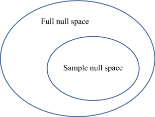
Not null enough: pseudo-null hypotheses in community ecology and comparative psychology

William Bausman & Marta Halina

Bayesian data analysis in population ecology: motivations, methods, and benefits

Robert M. Dorazio

The multiple-comparison trap and the Raven’s paradox—perils of using null hypothesis testing in environmental assessment

Song S. Qian & Thomas F. Cuffney

In species co-occurrence studies, when claiming that a species exists, occurs, or is present on an island, ecologists typically mean that the species has established a breeding population on that island instead of just having several vagile individuals.

For a detailed discussion of the differences between neutral models and null models, see Gotelli and McGill ( 2006 ).

In species co-occurrence studies, the null models constructed by different ecologists may be more or less different from each other. Even Connor and Simberloff themselves keep modifying their null models in later publications. Nevertheless, the version I will introduce here, which appears in one of their earliest and also most-cited publications on this subject, helps demonstrate the key features of null-model-based hypothesis testing.

For reviews of the technical issues in the construction of null models, see Gotelli and Graves ( 1996 ) and Sanderson and Pimm ( 2015 ).

Although the term “randomization test” is often used interchangeably with “permutation test,” actually they are different. A randomization test is based on random assignment involved in experimental design; the procedure of random assignment is conducted before empirical data are collected. By contrast, a permutation test is a nonparametric method of statistical hypothesis testing based on data resampling.

Bausman WC (2018) Modeling: neutral, null, and baseline. Philos Sci 85:594–616

Article   Google Scholar  

Bausman W, Halina M (2018) Not null enough: pseudo-null hypotheses in community ecology and comparative psychology. Biol Philos 33:1–20

Chase JM, Leibold MA (2003) Ecological niches: linking classical and contemporary approaches. University of Chicago Press, Chicago

Book   Google Scholar  

Colwell RK, Winkler DW (1984) A null model for null models in biogeography. In: Strong DR Jr, Simberloff D, Abele LG, Thistle AB (eds) Ecological communities: conceptual issues and the evidence. Princeton University Press, Princeton, pp 344–359

Chapter   Google Scholar  

Connor EF, Simberloff D (1979) The assembly of species communities: chance or competition? Ecology 60:1132–1140

Connor EF, Simberloff D (1983) Interspecific competition and species co-occurrence patterns on islands: null models and the evaluation of evidence. Oikos 41:455–465

Connor EF, Simberloff D (1984) Neutral models of species’ co-occurrence patterns. In: Strong DR Jr, Simberloff D, Abele LG, Thistle AB (eds) Ecological communities: conceptual issues and the evidence. Princeton University Press, Princeton, pp 316–331

Connor EF, Collins MD, Simberloff D (2013) The checkered history of checkerboard distributions. Ecology 94:2403–2414

Connor EF, Collins MD, Simberloff D (2015) The checkered history of checkerboard distributions: reply. Ecology 96:3388–3389

Diamond JM (1975) Assembly of species communities. In: Cody ML, Diamond JM (eds) Ecology and evolution of communities. Harvard University Press, Cambridge, pp 342–444

Google Scholar  

Diamond JM, Gilpin ME (1982) Examination of the “null” model of Connor and Simberloff for species co-occurrences on islands. Oecologia 52:64–74

Diamond J, Pimm SL, Sanderson JG (2015) The checkered history of checkerboard distributions: comment. Ecology 96:3386–3388

Fisher RA (1925) Statistical methods for research workers. Oliver and Boyd, Edinburgh

Fisher RA (1926) The arrangement of field experiments. J Minist Agric 33:503–513

Fisher RA (1935) The design of experiments. Oliver and Boyd, Edinburgh

Gilpin ME, Diamond JM (1984) Are species co-occurrences on islands non-random, and are null hypotheses useful in community ecology? In: Strong DR Jr, Simberloff D, Abele LG, Thistle AB (eds) Ecological communities: conceptual issues and the evidence. Princeton University Press, Princeton, pp 297–315

Gotelli NJ, Graves GR (1996) Null models in ecology. Smithsonian Institution Press, Washington

Gotelli NJ, McGill BJ (2006) Null versus neutral models: what’s the difference? Ecography 29:793–800

Harvey PH (1987) On the use of null hypotheses in biogeography. In: Nitechi MH, Hoffman A (eds) Neutral models in biology. Oxford University Press, New York, pp 109–118

Hubbell SP (2001) The unified neutral theory of biodiversity and biogeography. Princeton University Press, Princeton

Hubbell SP (2006) Neutral theory and the evolution of ecological equivalence. Ecology 87:1387–1398

Lewin R (1983) Santa Rosalia was a goat. Science 221:636–639

MacArthur R (1972) Geographical ecology: patterns in the distribution of species. Harper & Row, Publishers, Inc., New York

Rathcke BJ (1984) Patterns of flowering phenologies: testability and causal inference using a random model. In: Strong DR Jr, Simberloff D, Abele LG, Thistle AB (eds) Ecological communities: conceptual issues and the evidence. Princeton University Press, Princeton, pp 383–396

Rosindell J, Hubbell SP, Etienne RS (2011) The unified neutral theory of biodiversity and biogeography at age ten. Trends Ecol Evol 26:340–348

Sanderson JG, Pimm SL (2015) Patterns in nature: the analysis of species co-occurences. The University of Chicago Press, Chicago

Schelling TC (1978) Micromotives and macrobehavior. W. W. Norton & Company, New York

Sloep PB (1986) Null hypotheses in ecology: towards the dissolution of a controversy. Philos Sci 1:307–313

Sober E (1988) Reconstructing the past: parsimony, evolution, and inference. The MIT Press, Cambridge

Sober E (1994) Let’s Razor Ockham’s Razor. In: From a biological point of view. Cambridge University Press, Cambridge, pp 136–157

von Bertalanffy L (1968) General system theory: foundations, development, applications. George Braziller, New York

Download references

Acknowledgements

I wish to acknowledge the great help of Michael Weisberg, Erol Akçay, Jay Odenbaugh, and two anonymous reviewers for suggestions on improving the manuscript. An earlier draft of this article was also presented in the Philosophy of Science Reading Group at the University of Pennsylvania, the Salon of Philosophy of Science and Technology at Tsinghua University in Beijing, and PBDB 13 (Philosophy of Biology at Dolphin Beach) in Moruya, Australia. I want to thank the participants of these meetings, who asked valuable questions that inspired this article.

Author information

Authors and affiliations.

Department of Philosophy, University of Pennsylvania, Claudia Cohen Hall, Room 433, 249 S. 36th Street, Philadelphia, PA, 19104-6304, USA

Mingjun Zhang

You can also search for this author in PubMed   Google Scholar

Corresponding author

Correspondence to Mingjun Zhang .

Additional information

Publisher's note.

Springer Nature remains neutral with regard to jurisdictional claims in published maps and institutional affiliations.

Rights and permissions

Reprints and permissions

About this article

Zhang, M. The use and limitations of null-model-based hypothesis testing. Biol Philos 35 , 31 (2020). https://doi.org/10.1007/s10539-020-09748-0

Download citation

Received : 29 June 2019

Accepted : 13 April 2020

Published : 23 April 2020

DOI : https://doi.org/10.1007/s10539-020-09748-0

Share this article

Anyone you share the following link with will be able to read this content:

Sorry, a shareable link is not currently available for this article.

Provided by the Springer Nature SharedIt content-sharing initiative

• Null hypothesis
• Checkerboard distribution
• Interspecific competition
• Random colonization
• Control of variables
• Find a journal
• Publish with us
• Track your research