hypothesis for linear regression analysis

Statistics Made Easy

Understanding the Null Hypothesis for Linear Regression

Linear regression is a technique we can use to understand the relationship between one or more predictor variables and a response variable .

If we only have one predictor variable and one response variable, we can use simple linear regression , which uses the following formula to estimate the relationship between the variables:

ŷ = β 0 + β 1 x

• ŷ: The estimated response value.
• β 0 : The average value of y when x is zero.
• β 1 : The average change in y associated with a one unit increase in x.
• x: The value of the predictor variable.

Simple linear regression uses the following null and alternative hypotheses:

• H 0 : β 1 = 0
• H A : β 1 ≠ 0

The null hypothesis states that the coefficient β 1 is equal to zero. In other words, there is no statistically significant relationship between the predictor variable, x, and the response variable, y.

The alternative hypothesis states that β 1 is not equal to zero. In other words, there is a statistically significant relationship between x and y.

If we have multiple predictor variables and one response variable, we can use multiple linear regression , which uses the following formula to estimate the relationship between the variables:

ŷ = β 0 + β 1 x 1 + β 2 x 2 + … + β k x k

• β 0 : The average value of y when all predictor variables are equal to zero.
• β i : The average change in y associated with a one unit increase in x i .
• x i : The value of the predictor variable x i .

Multiple linear regression uses the following null and alternative hypotheses:

• H 0 : β 1 = β 2 = … = β k = 0
• H A : β 1 = β 2 = … = β k ≠ 0

The null hypothesis states that all coefficients in the model are equal to zero. In other words, none of the predictor variables have a statistically significant relationship with the response variable, y.

The alternative hypothesis states that not every coefficient is simultaneously equal to zero.

The following examples show how to decide to reject or fail to reject the null hypothesis in both simple linear regression and multiple linear regression models.

Example 1: Simple Linear Regression

Suppose a professor would like to use the number of hours studied to predict the exam score that students will receive in his class. He collects data for 20 students and fits a simple linear regression model.

The following screenshot shows the output of the regression model:

The fitted simple linear regression model is:

Exam Score = 67.1617 + 5.2503*(hours studied)

To determine if there is a statistically significant relationship between hours studied and exam score, we need to analyze the overall F value of the model and the corresponding p-value:

• Overall F-Value:  47.9952
• P-value:  0.000

Since this p-value is less than .05, we can reject the null hypothesis. In other words, there is a statistically significant relationship between hours studied and exam score received.

Example 2: Multiple Linear Regression

Suppose a professor would like to use the number of hours studied and the number of prep exams taken to predict the exam score that students will receive in his class. He collects data for 20 students and fits a multiple linear regression model.

The fitted multiple linear regression model is:

Exam Score = 67.67 + 5.56*(hours studied) – 0.60*(prep exams taken)

To determine if there is a jointly statistically significant relationship between the two predictor variables and the response variable, we need to analyze the overall F value of the model and the corresponding p-value:

• Overall F-Value:  23.46
• P-value:  0.00

Since this p-value is less than .05, we can reject the null hypothesis. In other words, hours studied and prep exams taken have a jointly statistically significant relationship with exam score.

Note: Although the p-value for prep exams taken (p = 0.52) is not significant, prep exams combined with hours studied has a significant relationship with exam score.

Additional Resources

Understanding the F-Test of Overall Significance in Regression How to Read and Interpret a Regression Table How to Report Regression Results How to Perform Simple Linear Regression in Excel How to Perform Multiple Linear Regression in Excel

Featured Posts

Hey there. My name is Zach Bobbitt. I have a Masters of Science degree in Applied Statistics and I’ve worked on machine learning algorithms for professional businesses in both healthcare and retail. I’m passionate about statistics, machine learning, and data visualization and I created Statology to be a resource for both students and teachers alike.  My goal with this site is to help you learn statistics through using simple terms, plenty of real-world examples, and helpful illustrations.

2 Replies to “Understanding the Null Hypothesis for Linear Regression”

Thank you Zach, this helped me on homework!

Great articles, Zach.

I would like to cite your work in a research paper.

Could you provide me with your last name and initials.

Leave a Reply Cancel reply

Your email address will not be published. Required fields are marked *

Join the Statology Community

Sign up to receive Statology's exclusive study resource: 100 practice problems with step-by-step solutions. Plus, get our latest insights, tutorials, and data analysis tips straight to your inbox!

By subscribing you accept Statology's Privacy Policy.

Linear regression - Hypothesis testing

by Marco Taboga , PhD

This lecture discusses how to perform tests of hypotheses about the coefficients of a linear regression model estimated by ordinary least squares (OLS).

Table of contents

Normal vs non-normal model

The linear regression model, matrix notation, tests of hypothesis in the normal linear regression model, test of a restriction on a single coefficient (t test), test of a set of linear restrictions (f test), tests based on maximum likelihood procedures (wald, lagrange multiplier, likelihood ratio), tests of hypothesis when the ols estimator is asymptotically normal, test of a restriction on a single coefficient (z test), test of a set of linear restrictions (chi-square test), learn more about regression analysis.

The lecture is divided in two parts:

in the first part, we discuss hypothesis testing in the normal linear regression model , in which the OLS estimator of the coefficients has a normal distribution conditional on the matrix of regressors;

in the second part, we show how to carry out hypothesis tests in linear regression analyses where the hypothesis of normality holds only in large samples (i.e., the OLS estimator can be proved to be asymptotically normal).

We also denote:

We now explain how to derive tests about the coefficients of the normal linear regression model.

It can be proved (see the lecture about the normal linear regression model ) that the assumption of conditional normality implies that:

How the acceptance region is determined depends not only on the desired size of the test , but also on whether the test is:

one-tailed (only one of the two things, i.e., either smaller or larger, is possible).

For more details on how to determine the acceptance region, see the glossary entry on critical values .

The F test is one-tailed .

A critical value in the right tail of the F distribution is chosen so as to achieve the desired size of the test.

Then, the null hypothesis is rejected if the F statistics is larger than the critical value.

In this section we explain how to perform hypothesis tests about the coefficients of a linear regression model when the OLS estimator is asymptotically normal.

As we have shown in the lecture on the properties of the OLS estimator , in several cases (i.e., under different sets of assumptions) it can be proved that:

These two properties are used to derive the asymptotic distribution of the test statistics used in hypothesis testing.

The test can be either one-tailed or two-tailed . The same comments made for the t-test apply here.

Like the F test, also the Chi-square test is usually one-tailed .

The desired size of the test is achieved by appropriately choosing a critical value in the right tail of the Chi-square distribution.

The null is rejected if the Chi-square statistics is larger than the critical value.

Want to learn more about regression analysis? Here are some suggestions:

R squared of a linear regression ;

Gauss-Markov theorem ;

Generalized Least Squares ;

Multicollinearity ;

Dummy variables ;

Selection of linear regression models

Partitioned regression ;

Ridge regression .

How to cite

Please cite as:

Taboga, Marco (2021). "Linear regression - Hypothesis testing", Lectures on probability theory and mathematical statistics. Kindle Direct Publishing. Online appendix. https://www.statlect.com/fundamentals-of-statistics/linear-regression-hypothesis-testing.

Most of the learning materials found on this website are now available in a traditional textbook format.

• F distribution
• Beta distribution
• Conditional probability
• Central Limit Theorem
• Binomial distribution
• Mean square convergence
• Delta method
• Almost sure convergence
• Mathematical tools
• Fundamentals of probability
• Probability distributions
• Asymptotic theory
• Fundamentals of statistics
• About Statlect
• Cookies, privacy and terms of use
• Loss function
• Almost sure
• Type I error
• Precision matrix
• Integrable variable
• To enhance your privacy,
• we removed the social buttons,
• but don't forget to share .

User Preferences

Content preview.

Arcu felis bibendum ut tristique et egestas quis:

• Ut enim ad minim veniam, quis nostrud exercitation ullamco laboris
• Duis aute irure dolor in reprehenderit in voluptate
• Excepteur sint occaecat cupidatat non proident

Keyboard Shortcuts

Lesson 1: simple linear regression, overview section  .

Simple linear regression is a statistical method that allows us to summarize and study relationships between two continuous (quantitative) variables. This lesson introduces the concept and basic procedures of simple linear regression.

• Distinguish between a deterministic relationship and a statistical relationship.
• Understand the concept of the least squares criterion.
• Interpret the intercept \(b_{0}\) and slope \(b_{1}\) of an estimated regression equation.
• Know how to obtain the estimates \(b_{0}\) and \(b_{1}\) from Minitab's fitted line plot and regression analysis output.
• Recognize the distinction between a population regression line and the estimated regression line.
• Summarize the four conditions that comprise the simple linear regression model.
• Know what the unknown population variance \(\sigma^{2}\) quantifies in the regression setting.
• Know how to obtain the estimated MSE of the unknown population variance \(\sigma^{2 }\) from Minitab's fitted line plot and regression analysis output.
• Know that the coefficient of determination (\(R^2\)) and the correlation coefficient (r) are measures of linear association. That is, they can be 0 even if there is a perfect nonlinear association.
• Know how to interpret the \(R^2\) value.
• Understand the cautions necessary in using the \(R^2\) value as a way of assessing the strength of the linear association.
• Know how to calculate the correlation coefficient r from the \(R^2\) value.
• Know what various correlation coefficient values mean. There is no meaningful interpretation for the correlation coefficient as there is for the \(R^2\) value.

Lesson 1 Code Files Section  

STAT501_Lesson01.zip

• bldgstories.txt
• carstopping.txt
• drugdea.txt
• fev_dat.txt
• heightgpa.txt
• husbandwife.txt
• oldfaithful.txt
• poverty.txt
• practical.txt
• signdist.txt
• skincancer.txt
• student_height_weight.txt

• Prompt Library
• DS/AI Trends
• Stats Tools
• Interview Questions
• Generative AI
• Machine Learning
• Deep Learning

Linear regression hypothesis testing: Concepts, Examples

In relation to machine learning , linear regression is defined as a predictive modeling technique that allows us to build a model which can help predict continuous response variables as a function of a linear combination of explanatory or predictor variables. While training linear regression models, we need to rely on hypothesis testing in relation to determining the relationship between the response and predictor variables. In the case of the linear regression model, two types of hypothesis testing are done. They are T-tests and F-tests . In other words, there are two types of statistics that are used to assess whether linear regression models exist representing response and predictor variables. They are t-statistics and f-statistics. As data scientists , it is of utmost importance to determine if linear regression is the correct choice of model for our particular problem and this can be done by performing hypothesis testing related to linear regression response and predictor variables. Many times, it is found that these concepts are not very clear with a lot many data scientists. In this blog post, we will discuss linear regression and hypothesis testing related to t-statistics and f-statistics . We will also provide an example to help illustrate how these concepts work.

Table of Contents

What are linear regression models?

A linear regression model can be defined as the function approximation that represents a continuous response variable as a function of one or more predictor variables. While building a linear regression model, the goal is to identify a linear equation that best predicts or models the relationship between the response or dependent variable and one or more predictor or independent variables.

There are two different kinds of linear regression models. They are as follows:

• Simple or Univariate linear regression models : These are linear regression models that are used to build a linear relationship between one response or dependent variable and one predictor or independent variable. The form of the equation that represents a simple linear regression model is Y=mX+b, where m is the coefficients of the predictor variable and b is bias. When considering the linear regression line, m represents the slope and b represents the intercept.
• Multiple or Multi-variate linear regression models : These are linear regression models that are used to build a linear relationship between one response or dependent variable and more than one predictor or independent variable. The form of the equation that represents a multiple linear regression model is Y=b0+b1X1+ b2X2 + … + bnXn, where bi represents the coefficients of the ith predictor variable. In this type of linear regression model, each predictor variable has its own coefficient that is used to calculate the predicted value of the response variable.

While training linear regression models, the requirement is to determine the coefficients which can result in the best-fitted linear regression line. The learning algorithm used to find the most appropriate coefficients is known as least squares regression . In the least-squares regression method, the coefficients are calculated using the least-squares error function. The main objective of this method is to minimize or reduce the sum of squared residuals between actual and predicted response values. The sum of squared residuals is also called the residual sum of squares (RSS). The outcome of executing the least-squares regression method is coefficients that minimize the linear regression cost function .

The residual e of the ith observation is represented as the following where [latex]Y_i[/latex] is the ith observation and [latex]\hat{Y_i}[/latex] is the prediction for ith observation or the value of response variable for ith observation.

[latex]e_i = Y_i – \hat{Y_i}[/latex]

The residual sum of squares can be represented as the following:

[latex]RSS = e_1^2 + e_2^2 + e_3^2 + … + e_n^2[/latex]

The least-squares method represents the algorithm that minimizes the above term, RSS.

Once the coefficients are determined, can it be claimed that these coefficients are the most appropriate ones for linear regression? The answer is no. After all, the coefficients are only the estimates and thus, there will be standard errors associated with each of the coefficients.  Recall that the standard error is used to calculate the confidence interval in which the mean value of the population parameter would exist. In other words, it represents the error of estimating a population parameter based on the sample data. The value of the standard error is calculated as the standard deviation of the sample divided by the square root of the sample size. The formula below represents the standard error of a mean.

[latex]SE(\mu) = \frac{\sigma}{\sqrt(N)}[/latex]

Thus, without analyzing aspects such as the standard error associated with the coefficients, it cannot be claimed that the linear regression coefficients are the most suitable ones without performing hypothesis testing. This is where hypothesis testing is needed . Before we get into why we need hypothesis testing with the linear regression model, let’s briefly learn about what is hypothesis testing?

Train a Multiple Linear Regression Model using R

Before getting into understanding the hypothesis testing concepts in relation to the linear regression model, let’s train a multi-variate or multiple linear regression model and print the summary output of the model which will be referred to, in the next section. 

The data used for creating a multi-linear regression model is BostonHousing which can be loaded in RStudioby installing mlbench package. The code is shown below:

install.packages(“mlbench”) library(mlbench) data(“BostonHousing”)

Once the data is loaded, the code shown below can be used to create the linear regression model.

attach(BostonHousing) BostonHousing.lm <- lm(log(medv) ~ crim + chas + rad + lstat) summary(BostonHousing.lm)

Executing the above command will result in the creation of a linear regression model with the response variable as medv and predictor variables as crim, chas, rad, and lstat. The following represents the details related to the response and predictor variables:

• log(medv) : Log of the median value of owner-occupied homes in USD 1000’s
• crim : Per capita crime rate by town
• chas : Charles River dummy variable (= 1 if tract bounds river; 0 otherwise)
• rad : Index of accessibility to radial highways
• lstat : Percentage of the lower status of the population

The following will be the output of the summary command that prints the details relating to the model including hypothesis testing details for coefficients (t-statistics) and the model as a whole (f-statistics) 

Hypothesis tests & Linear Regression Models

Hypothesis tests are the statistical procedure that is used to test a claim or assumption about the underlying distribution of a population based on the sample data. Here are key steps of doing hypothesis tests with linear regression models:

• Hypothesis formulation for T-tests: In the case of linear regression, the claim is made that there exists a relationship between response and predictor variables, and the claim is represented using the non-zero value of coefficients of predictor variables in the linear equation or regression model. This is formulated as an alternate hypothesis. Thus, the null hypothesis is set that there is no relationship between response and the predictor variables . Hence, the coefficients related to each of the predictor variables is equal to zero (0). So, if the linear regression model is Y = a0 + a1x1 + a2x2 + a3x3, then the null hypothesis for each test states that a1 = 0, a2 = 0, a3 = 0 etc. For all the predictor variables, individual hypothesis testing is done to determine whether the relationship between response and that particular predictor variable is statistically significant based on the sample data used for training the model. Thus, if there are, say, 5 features, there will be five hypothesis tests and each will have an associated null and alternate hypothesis.
• Hypothesis formulation for F-test : In addition, there is a hypothesis test done around the claim that there is a linear regression model representing the response variable and all the predictor variables. The null hypothesis is that the linear regression model does not exist . This essentially means that the value of all the coefficients is equal to zero. So, if the linear regression model is Y = a0 + a1x1 + a2x2 + a3x3, then the null hypothesis states that a1 = a2 = a3 = 0.
• F-statistics for testing hypothesis for linear regression model : F-test is used to test the null hypothesis that a linear regression model does not exist, representing the relationship between the response variable y and the predictor variables x1, x2, x3, x4 and x5. The null hypothesis can also be represented as x1 = x2 = x3 = x4 = x5 = 0. F-statistics is calculated as a function of sum of squares residuals for restricted regression (representing linear regression model with only intercept or bias and all the values of coefficients as zero) and sum of squares residuals for unrestricted regression (representing linear regression model). In the above diagram, note the value of f-statistics as 15.66 against the degrees of freedom as 5 and 194. 
• Evaluate t-statistics against the critical value/region : After calculating the value of t-statistics for each coefficient, it is now time to make a decision about whether to accept or reject the null hypothesis. In order for this decision to be made, one needs to set a significance level, which is also known as the alpha level. The significance level of 0.05 is usually set for rejecting the null hypothesis or otherwise. If the value of t-statistics fall in the critical region, the null hypothesis is rejected. Or, if the p-value comes out to be less than 0.05, the null hypothesis is rejected.
• Evaluate f-statistics against the critical value/region : The value of F-statistics and the p-value is evaluated for testing the null hypothesis that the linear regression model representing response and predictor variables does not exist. If the value of f-statistics is more than the critical value at the level of significance as 0.05, the null hypothesis is rejected. This means that the linear model exists with at least one valid coefficients. 
• Draw conclusions : The final step of hypothesis testing is to draw a conclusion by interpreting the results in terms of the original claim or hypothesis. If the null hypothesis of one or more predictor variables is rejected, it represents the fact that the relationship between the response and the predictor variable is not statistically significant based on the evidence or the sample data we used for training the model. Similarly, if the f-statistics value lies in the critical region and the value of the p-value is less than the alpha value usually set as 0.05, one can say that there exists a linear regression model.

Why hypothesis tests for linear regression models?

The reasons why we need to do hypothesis tests in case of a linear regression model are following:

• By creating the model, we are establishing a new truth (claims) about the relationship between response or dependent variable with one or more predictor or independent variables. In order to justify the truth, there are needed one or more tests. These tests can be termed as an act of testing the claim (or new truth) or in other words, hypothesis tests.
• One kind of test is required to test the relationship between response and each of the predictor variables (hence, T-tests)
• Another kind of test is required to test the linear regression model representation as a whole. This is called F-test.

While training linear regression models, hypothesis testing is done to determine whether the relationship between the response and each of the predictor variables is statistically significant or otherwise. The coefficients related to each of the predictor variables is determined. Then, individual hypothesis tests are done to determine whether the relationship between response and that particular predictor variable is statistically significant based on the sample data used for training the model. If at least one of the null hypotheses is rejected, it represents the fact that there exists no relationship between response and that particular predictor variable. T-statistics is used for performing the hypothesis testing because the standard deviation of the sampling distribution is unknown. The value of t-statistics is compared with the critical value from the t-distribution table in order to make a decision about whether to accept or reject the null hypothesis regarding the relationship between the response and predictor variables. If the value falls in the critical region, then the null hypothesis is rejected which means that there is no relationship between response and that predictor variable. In addition to T-tests, F-test is performed to test the null hypothesis that the linear regression model does not exist and that the value of all the coefficients is zero (0). Learn more about the linear regression and t-test in this blog – Linear regression t-test: formula, example .

Recent Posts

• Pricing Analytics in Banking: Strategies, Examples - May 15, 2024
• How to Learn Effectively: A Holistic Approach - May 13, 2024
• How to Choose Right Statistical Tests: Examples - May 13, 2024

Ajitesh Kumar

One response.

Very informative

Leave a Reply Cancel reply

Your email address will not be published. Required fields are marked *

• Search for:
• Excellence Awaits: IITs, NITs & IIITs Journey

ChatGPT Prompts (250+)

• Generate Design Ideas for App
• Expand Feature Set of App
• Create a User Journey Map for App
• Generate Visual Design Ideas for App
• Generate a List of Competitors for App
• Pricing Analytics in Banking: Strategies, Examples
• How to Learn Effectively: A Holistic Approach
• How to Choose Right Statistical Tests: Examples
• Data Lakehouses Fundamentals & Examples
• Machine Learning Lifecycle: Data to Deployment Example

Data Science / AI Trends

• • Prepend any arxiv.org link with talk2 to load the paper into a responsive chat application
• • Custom LLM and AI Agents (RAG) On Structured + Unstructured Data - AI Brain For Your Organization
• • Guides, papers, lecture, notebooks and resources for prompt engineering
• • Common tricks to make LLMs efficient and stable
• • Machine learning in finance

Free Online Tools

• Create Scatter Plots Online for your Excel Data
• Histogram / Frequency Distribution Creation Tool
• Online Pie Chart Maker Tool
• Z-test vs T-test Decision Tool
• Independent samples t-test calculator

Recent Comments

I found it very helpful. However the differences are not too understandable for me

Very Nice Explaination. Thankyiu very much,

in your case E respresent Member or Oraganization which include on e or more peers?

Such a informative post. Keep it up

Thank you....for your support. you given a good solution for me.

Regression Analysis

• Reference work entry
• First Online: 03 December 2021
• Cite this reference work entry

• Bernd Skiera 4 ,
• Jochen Reiner 4 &
• Sönke Albers 5  

7624 Accesses

3 Citations

Linear regression analysis is one of the most important statistical methods. It examines the linear relationship between a metric-scaled dependent variable (also called endogenous, explained, response, or predicted variable) and one or more metric-scaled independent variables (also called exogenous, explanatory, control, or predictor variable). We illustrate how regression analysis work and how it supports marketing decisions, e.g., the derivation of an optimal marketing mix. We also outline how to use linear regression analysis to estimate nonlinear functions such as a multiplicative sales response function. Furthermore, we show how to use the results of a regression to calculate elasticities and to identify outliers and discuss in details the problems that occur in case of autocorrelation, multicollinearity and heteroscedasticity. We use a numerical example to illustrate in detail all calculations and use this numerical example to outline the problems that occur in case of endogeneity.

This is a preview of subscription content, log in via an institution to check access.

Access this chapter

• Available as PDF
• Read on any device
• Instant download
• Own it forever
• Available as EPUB and PDF
• Durable hardcover edition
• Dispatched in 3 to 5 business days
• Free shipping worldwide - see info

Tax calculation will be finalised at checkout

Purchases are for personal use only

Institutional subscriptions

Similar content being viewed by others

Estimation and Testing

Albers, S. (2012). Optimizable and implementable aggregate response modeling for marketing decision support. International Journal of Research in Marketing, 29 (2), 111–122.

Article   Google Scholar  

Albers, S., Mantrala, M. K., & Sridhar, S. (2010). Personal selling elasticities: A meta-analysis. Journal of Marketing Research, 47 (5), 840–853.

Assmus, G., Farley, J. W., & Lehmann, D. R. (1984). How advertising affects sales: A meta-analysis of econometric results. Journal of Marketing Research, 21 (1), 65–74.

Bijmolt, T. H. A., van Heerde, H., & Pieters, R. G. M. (2005). New empirical generalizations on the determinants of price elasticity. Journal of Marketing Research, 42 (2), 141–156.

Chatterjee, S., & Hadi, A. S. (1986). Influential observations, high leverage points, and outliers in linear regressions. Statistical Science, 1 (3), 379–416.

Google Scholar  

Greene, W. H. (2008). Econometric analysis (6th ed.). Upper Saddle River: Pearson.

Gujarati, D. N. (2003). Basic econometrics (4th ed.). New York: McGraw Hill.

Hair, J. F., Black, W. C., Babin, J. B., & Anderson, R. E. (2014). Multivariate data analysis (7th ed.). Upper Saddle River: Pearson.

Hair, J. F., Hult, G. T. M., Ringle, C. M., & Sarstedt, M. (2017). A primer on partial least squares structural equation modeling (PLS-SEM) (2nd ed.). Thousand Oaks: Sage.

Hanssens, D. M., Parsons, L. J., & Schultz, R. L. (1990). Market response models: Econometric and time series analysis . Boston: Springer.

Hsiao, C. (2014). Analysis of panel data (3rd ed.). Cambridge: Cambridge University Press.

Book   Google Scholar  

Irwin, J. R., & McClelland, G. H. (2001). Misleading heuristics and moderated multiple regression models. Journal of Marketing Research, 38 (1), 100–109.

Koutsoyiannis, A. (1977). Theory of econometrics (2nd ed.). Houndmills: MacMillan.

Laurent, G. (2013). EMAC distinguished marketing scholar 2012: Respect the data! International Journal of Research in Marketing, 30 (4), 323–334.

Leeflang, P. S. H., Wittink, D. R., Wedel, M., & Neart, P. A. (2000). Building models for marketing decisions . Berlin: Kluwer.

Lodish, L. L., Abraham, M. M., Kalmenson, S., Livelsberger, J., Lubetkin, B., Richardson, B., & Stevens, M. E. (1995). How TV advertising works: A meta-analysis of 389 real world split cable T. V. advertising experiments. Journal of Marketing Research, 32 (2), 125–139.

Pindyck, R. S., & Rubenfeld, D. (1998). Econometric models and econometric forecasts (4th ed.). New York: McGraw-Hill.

Sethuraman, R., Tellis, G. J., & Briesch, R. A. (2011). How well does advertising work? Generalizations from meta-analysis of brand advertising elasticities. Journal of Marketing Research, 48 (3), 457–471.

Snijders, T. A. B., & Bosker, R. J. (2012). Multilevel analysis: An introduction to basic and advanced multilevel modeling (2nd ed.). London: Sage.

Stock, J., & Watson, M. (2015). Introduction to econometrics (3rd ed.). Upper Saddle River: Pearson.

Tellis, G. J. (1988). The price sensitivity of selective demand: A meta-analysis of econometric models of sales. Journal of Marketing Research, 25 (4), 391–404.

White, H. (1980). A heteroskedasticity-consistent covariance matrix estimator and a direct test for heteroskedasticity. Econometrica, 48 (4), 817–838.

Wooldridge, J. M. (2009). Introductory econometrics: A modern approach (4th ed.). Mason: South-Western Cengage.

Download references

Author information

Authors and affiliations.

Goethe University Frankfurt, Frankfurt, Germany

Bernd Skiera & Jochen Reiner

Kuehne Logistics University, Hamburg, Germany

Sönke Albers

You can also search for this author in PubMed   Google Scholar

Corresponding author

Correspondence to Bernd Skiera .

Editor information

Editors and affiliations.

Department of Business-to-Business Marketing, Sales, and Pricing, University of Mannheim, Mannheim, Germany

Christian Homburg

Department of Marketing & Sales Research Group, Karlsruhe Institute of Technology (KIT), Karlsruhe, Germany

Martin Klarmann

Marketing & Sales Department, University of Mannheim, Mannheim, Germany

Arnd Vomberg

Rights and permissions

Reprints and permissions

Copyright information

© 2022 Springer Nature Switzerland AG

About this entry

Cite this entry.

Skiera, B., Reiner, J., Albers, S. (2022). Regression Analysis. In: Homburg, C., Klarmann, M., Vomberg, A. (eds) Handbook of Market Research. Springer, Cham. https://doi.org/10.1007/978-3-319-57413-4_17

Download citation

DOI : https://doi.org/10.1007/978-3-319-57413-4_17

Published : 03 December 2021

Publisher Name : Springer, Cham

Print ISBN : 978-3-319-57411-0

Online ISBN : 978-3-319-57413-4

eBook Packages : Business and Management Reference Module Humanities and Social Sciences Reference Module Business, Economics and Social Sciences

Share this entry

Anyone you share the following link with will be able to read this content:

Sorry, a shareable link is not currently available for this article.

Provided by the Springer Nature SharedIt content-sharing initiative

• Publish with us

Policies and ethics

• Find a journal
• Track your research

Browse Course Material

Course info, instructors.

• Prof. Cynthia Rudin
• Allison Chang
• Dimitrios Bisias

Departments

• Sloan School of Management
• Institute for Data, Systems, and Society

As Taught In

• Data Mining
• Probability and Statistics

Learning Resource Types

Statistical thinking and data analysis, course description.

You are leaving MIT OpenCourseWare

Linear Regression Analysis using SPSS Statistics

Introduction.

Linear regression is the next step up after correlation. It is used when we want to predict the value of a variable based on the value of another variable. The variable we want to predict is called the dependent variable (or sometimes, the outcome variable). The variable we are using to predict the other variable's value is called the independent variable (or sometimes, the predictor variable). For example, you could use linear regression to understand whether exam performance can be predicted based on revision time; whether cigarette consumption can be predicted based on smoking duration; and so forth. If you have two or more independent variables, rather than just one, you need to use multiple regression .

This "quick start" guide shows you how to carry out linear regression using SPSS Statistics, as well as interpret and report the results from this test. However, before we introduce you to this procedure, you need to understand the different assumptions that your data must meet in order for linear regression to give you a valid result. We discuss these assumptions next.

SPSS Statistics

Assumptions.

When you choose to analyse your data using linear regression, part of the process involves checking to make sure that the data you want to analyse can actually be analysed using linear regression. You need to do this because it is only appropriate to use linear regression if your data "passes" seven assumptions that are required for linear regression to give you a valid result. In practice, checking for these seven assumptions just adds a little bit more time to your analysis, requiring you to click a few more buttons in SPSS Statistics when performing your analysis, as well as think a little bit more about your data, but it is not a difficult task.

Before we introduce you to these seven assumptions, do not be surprised if, when analysing your own data using SPSS Statistics, one or more of these assumptions is violated (i.e., not met). This is not uncommon when working with real-world data rather than textbook examples, which often only show you how to carry out linear regression when everything goes well! However, don’t worry. Even when your data fails certain assumptions, there is often a solution to overcome this. First, let’s take a look at these seven assumptions:

• Assumption #1: Your dependent variable should be measured at the continuous level (i.e., it is either an interval or ratio variable). Examples of continuous variables include revision time (measured in hours), intelligence (measured using IQ score), exam performance (measured from 0 to 100), weight (measured in kg), and so forth. You can learn more about interval and ratio variables in our article: Types of Variable .
• Assumption #2: Your independent variable should also be measured at the continuous level (i.e., it is either an interval or ratio variable). See the bullet above for examples of continuous variables.

• Assumption #5: You should have independence of observations , which you can easily check using the Durbin-Watson statistic, which is a simple test to run using SPSS Statistics. We explain how to interpret the result of the Durbin-Watson statistic in our enhanced linear regression guide.

• Assumption #7: Finally, you need to check that the residuals (errors) of the regression line are approximately normally distributed (we explain these terms in our enhanced linear regression guide). Two common methods to check this assumption include using either a histogram (with a superimposed normal curve) or a Normal P-P Plot. Again, in our enhanced linear regression guide, we: (a) show you how to check this assumption using SPSS Statistics, whether you use a histogram (with superimposed normal curve) or Normal P-P Plot; (b) explain how to interpret these diagrams; and (c) provide a possible solution if your data fails to meet this assumption.

You can check assumptions #3, #4, #5, #6 and #7 using SPSS Statistics. Assumptions #3 should be checked first, before moving onto assumptions #4, #5, #6 and #7. We suggest testing the assumptions in this order because assumptions #3, #4, #5, #6 and #7 require you to run the linear regression procedure in SPSS Statistics first, so it is easier to deal with these after checking assumption #1 and #2. Just remember that if you do not run the statistical tests on these assumptions correctly, the results you get when running a linear regression might not be valid. This is why we dedicate a number of sections of our enhanced linear regression guide to help you get this right. You can find out more about our enhanced content as a whole on our Features: Overview page, or more specifically, learn how we help with testing assumptions on our Features: Assumptions page.

In the section, Procedure , we illustrate the SPSS Statistics procedure to perform a linear regression assuming that no assumptions have been violated. First, we introduce the example that is used in this guide.

A salesperson for a large car brand wants to determine whether there is a relationship between an individual's income and the price they pay for a car. As such, the individual's "income" is the independent variable and the "price" they pay for a car is the dependent variable. The salesperson wants to use this information to determine which cars to offer potential customers in new areas where average income is known.

Setup in SPSS Statistics

In SPSS Statistics, we created two variables so that we could enter our data: Income (the independent variable), and Price (the dependent variable). It can also be useful to create a third variable, caseno , to act as a chronological case number. This third variable is used to make it easy for you to eliminate cases (e.g., significant outliers) that you have identified when checking for assumptions. However, we do not include it in the SPSS Statistics procedure that follows because we assume that you have already checked these assumptions. In our enhanced linear regression guide, we show you how to correctly enter data in SPSS Statistics to run a linear regression when you are also checking for assumptions. You can learn about our enhanced data setup content on our Features: Data Setup page. Alternately, see our generic, "quick start" guide: Entering Data in SPSS Statistics .

Test Procedure in SPSS Statistics

The five steps below show you how to analyse your data using linear regression in SPSS Statistics when none of the seven assumptions in the previous section, Assumptions , have been violated. At the end of these four steps, we show you how to interpret the results from your linear regression. If you are looking for help to make sure your data meets assumptions #3, #4, #5, #6 and #7, which are required when using linear regression and can be tested using SPSS Statistics, you can learn more about our enhanced guides on our Features: Overview page.

Note: The procedure that follows is identical for SPSS Statistics versions 18 to 28 , as well as the subscription version of SPSS Statistics, with version 28 and the subscription version being the latest versions of SPSS Statistics. However, in version 27 and the subscription version , SPSS Statistics introduced a new look to their interface called " SPSS Light ", replacing the previous look for versions 26 and earlier versions , which was called " SPSS Standard ". Therefore, if you have SPSS Statistics versions 27 or 28 (or the subscription version of SPSS Statistics), the images that follow will be light grey rather than blue. However, the procedure is identical .

Published with written permission from SPSS Statistics, IBM Corporation.

You will be presented with the Linear Regression dialogue box:

Access all 96 SPSS Statistics guides in Laerd Statistics

Output of Linear Regression Analysis

SPSS Statistics will generate quite a few tables of output for a linear regression. In this section, we show you only the three main tables required to understand your results from the linear regression procedure, assuming that no assumptions have been violated. A complete explanation of the output you have to interpret when checking your data for the six assumptions required to carry out linear regression is provided in our enhanced guide. This includes relevant scatterplots, histogram (with superimposed normal curve), Normal P-P Plot, casewise diagnostics and the Durbin-Watson statistic. Below, we focus on the results for the linear regression analysis only.

The first table of interest is the Model Summary table, as shown below:

This table provides the R and R 2 values. The R value represents the simple correlation and is 0.873 (the " R " Column), which indicates a high degree of correlation. The R 2 value (the " R Square " column) indicates how much of the total variation in the dependent variable, Price , can be explained by the independent variable, Income . In this case, 76.2% can be explained, which is very large.

The next table is the ANOVA table, which reports how well the regression equation fits the data (i.e., predicts the dependent variable) and is shown below:

This table indicates that the regression model predicts the dependent variable significantly well. How do we know this? Look at the " Regression " row and go to the " Sig. " column. This indicates the statistical significance of the regression model that was run. Here, p < 0.0005, which is less than 0.05, and indicates that, overall, the regression model statistically significantly predicts the outcome variable (i.e., it is a good fit for the data).

The Coefficients table provides us with the necessary information to predict price from income, as well as determine whether income contributes statistically significantly to the model (by looking at the " Sig. " column). Furthermore, we can use the values in the " B " column under the " Unstandardized Coefficients " column, as shown below:

to present the regression equation as:

Price = 8287 + 0.564(Income)

If you are unsure how to interpret regression equations or how to use them to make predictions, we discuss this in our enhanced linear regression guide. We also show you how to write up the results from your assumptions tests and linear regression output if you need to report this in a dissertation/thesis, assignment or research report. We do this using the Harvard and APA styles. You can learn more about our enhanced content on our Features: Overview page.

We also have a "quick start" guide on how to perform a linear regression analysis in Stata .

Save 10% on All AnalystPrep 2024 Study Packages with Coupon Code BLOG10 .

• Payment Plans
• Product List
• Partnerships

• Try Free Trial
• Study Packages
• Levels I, II & III Lifetime Package
• Video Lessons
• Study Notes
• Practice Questions
• Levels II & III Lifetime Package
• About the Exam
• About your Instructor
• Part I Study Packages
• Part I & Part II Lifetime Package
• Part II Study Packages
• Exams P & FM Lifetime Package
• Quantitative Questions
• Verbal Questions
• Data Insight Questions
• Live Tutoring
• About your Instructors
• EA Practice Questions
• Data Sufficiency Questions
• Integrated Reasoning Questions

Hypothesis Testing in Regression Analysis

Hypothesis testing is used to confirm if the estimated regression coefficients bear any statistical significance.  Either the confidence interval approach or the t-test approach can be used in hypothesis testing. In this section, we will explore the t-test approach.

The t-test Approach

The following are the steps followed in the performance of the t-test:

• Set the significance level for the test.
• Formulate the null and the alternative hypotheses.

$$t=\frac{\widehat{b_1}-b_1}{s_{\widehat{b_1}}}$$

\(b_1\) = True slope coefficient.

\(\widehat{b_1}\) = Point estimate for \(b_1\)

\(b_1 s_{\widehat{b_1\ }}\) = Standard error of the regression coefficient.

• Compare the absolute value of the t-statistic to the critical t-value (t_c). Reject the null hypothesis if the absolute value of the t-statistic is greater than the critical t-value i.e., \(t\ >\ +\ t_{critical}\ or\ t\ <\ –t_{\text{critical}}\).

Example: Hypothesis Testing of the Significance of Regression Coefficients

An analyst generates the following output from the regression analysis of inflation on unemployment:

$$\small{\begin{array}{llll}\hline{}& \textbf{Regression Statistics} &{}&{}\\ \hline{}& \text{Multiple R} & 0.8766 &{} \\ {}& \text{R Square} & 0.7684 &{} \\ {}& \text{Adjusted R Square} & 0.7394 & {}\\ {}& \text{Standard Error} & 0.0063 &{}\\ {}& \text{Observations} & 10 &{}\\ \hline {}& & & \\ \hline{} & \textbf{Coefficients} & \textbf{Standard Error} & \textbf{t-Stat}\\ \hline \text{Intercept} & 0.0710 & 0.0094 & 7.5160 \\\text{Forecast (Slope)} & -0.9041 & 0.1755 & -5.1516\\ \hline\end{array}}$$

At the 5% significant level, test the null hypothesis that the slope coefficient is significantly different from one, that is,

$$ H_{0}: b_{1} = 1\ vs. \ H_{a}: b_{1}≠1 $$

The calculated t-statistic, \(\text{t}=\frac{\widehat{b_{1}}-b_1}{\widehat{S_{b_{1}}}}\) is equal to:

$$\begin{align*}\text{t}& = \frac{-0.9041-1}{0.1755}\\& = -10.85\end{align*}$$

The critical two-tail t-values from the table with \(n-2=8\) degrees of freedom are:

$$\text{t}_{c}=±2.306$$

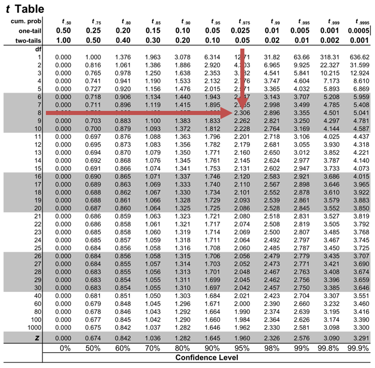
Notice that \(|t|>t_{c}\) i.e., (\(10.85>2.306\))

Therefore, we reject the null hypothesis and conclude that the estimated slope coefficient is statistically different from one.

Note that we used the confidence interval approach and arrived at the same conclusion.

Question Neeth Shinu, CFA, is forecasting price elasticity of supply for a certain product. Shinu uses the quantity of the product supplied for the past 5months as the dependent variable and the price per unit of the product as the independent variable. The regression results are shown below. $$\small{\begin{array}{lccccc}\hline \textbf{Regression Statistics} & & & & & \\ \hline \text{Multiple R} & 0.9971 & {}& {}&{}\\ \text{R Square} & 0.9941 & & & \\ \text{Adjusted R Square} & 0.9922 & & & & \\ \text{Standard Error} & 3.6515 & & & \\ \text{Observations} & 5 & & & \\ \hline {}& \textbf{Coefficients} & \textbf{Standard Error} & \textbf{t Stat} & \textbf{P-value}\\ \hline\text{Intercept} & -159 & 10.520 & (15.114) & 0.001\\ \text{Slope} & 0.26 & 0.012 & 22.517 & 0.000\\ \hline\end{array}}$$ Which of the following most likely reports the correct value of the t-statistic for the slope and most accurately evaluates its statistical significance with 95% confidence?     A. \(t=21.67\); slope is significantly different from zero.     B. \(t= 3.18\); slope is significantly different from zero.     C. \(t=22.57\); slope is not significantly different from zero. Solution The correct answer is A . The t-statistic is calculated using the formula: $$\text{t}=\frac{\widehat{b_{1}}-b_1}{\widehat{S_{b_{1}}}}$$ Where: \(b_{1}\) = True slope coefficient \(\widehat{b_{1}}\) = Point estimator for \(b_{1}\) \(\widehat{S_{b_{1}}}\) = Standard error of the regression coefficient $$\begin{align*}\text{t}&=\frac{0.26-0}{0.012}\\&=21.67\end{align*}$$ The critical two-tail t-values from the t-table with \(n-2 = 3\) degrees of freedom are: $$t_{c}=±3.18$$ Notice that \(|t|>t_{c}\) (i.e \(21.67>3.18\)). Therefore, the null hypothesis can be rejected. Further, we can conclude that the estimated slope coefficient is statistically different from zero.

Offered by AnalystPrep

Analysis of Variance (ANOVA)

Predicted value of a dependent variable, unimodal distribution – locations of ....

A unimodal distribution is a distribution that has one clear peak. The values... Read More

Assumptions Underlying Linear Regression

Assume that we have samples of size \(n\) for dependent variable \(Y\) and... Read More

Time Value of Money With Different Fre ...

Time value of money calculations allow us to establish the future value of... Read More

Measures of Central Tendency

Measures of central tendency are values that tend to occur at the center... Read More

An official website of the United States government

The .gov means it’s official. Federal government websites often end in .gov or .mil. Before sharing sensitive information, make sure you’re on a federal government site.

The site is secure. The https:// ensures that you are connecting to the official website and that any information you provide is encrypted and transmitted securely.

• Publications
• Account settings

Preview improvements coming to the PMC website in October 2024. Learn More or Try it out now .

• Advanced Search
• Journal List
• Dtsch Arztebl Int
• v.107(44); 2010 Nov

Linear Regression Analysis

Astrid schneider.

1 Departrment of Medical Biometrics, Epidemiology, and Computer Sciences, Johannes Gutenberg University, Mainz, Germany

Gerhard Hommel

Maria blettner.

Regression analysis is an important statistical method for the analysis of medical data. It enables the identification and characterization of relationships among multiple factors. It also enables the identification of prognostically relevant risk factors and the calculation of risk scores for individual prognostication.

This article is based on selected textbooks of statistics, a selective review of the literature, and our own experience.

After a brief introduction of the uni- and multivariable regression models, illustrative examples are given to explain what the important considerations are before a regression analysis is performed, and how the results should be interpreted. The reader should then be able to judge whether the method has been used correctly and interpret the results appropriately.

The performance and interpretation of linear regression analysis are subject to a variety of pitfalls, which are discussed here in detail. The reader is made aware of common errors of interpretation through practical examples. Both the opportunities for applying linear regression analysis and its limitations are presented.

The purpose of statistical evaluation of medical data is often to describe relationships between two variables or among several variables. For example, one would like to know not just whether patients have high blood pressure, but also whether the likelihood of having high blood pressure is influenced by factors such as age and weight. The variable to be explained (blood pressure) is called the dependent variable, or, alternatively, the response variable; the variables that explain it (age, weight) are called independent variables or predictor variables. Measures of association provide an initial impression of the extent of statistical dependence between variables. If the dependent and independent variables are continuous, as is the case for blood pressure and weight, then a correlation coefficient can be calculated as a measure of the strength of the relationship between them ( box 1 ).

Interpretation of the correlation coefficient (r)

Spearman’s coefficient:

Describes a monotone relationship

A monotone relationship is one in which the dependent variable either rises or sinks continuously as the independent variable rises.

Pearson’s correlation coefficient:

Describes a linear relationship

Interpretation/meaning:

Correlation coefficients provide information about the strength and direction of a relationship between two continuous variables. No distinction between the explaining variable and the variable to be explained is necessary:

• r = ± 1: perfect linear and monotone relationship. The closer r is to 1 or –1, the stronger the relationship.
• r = 0: no linear or monotone relationship
• r < 0: negative, inverse relationship (high values of one variable tend to occur together with low values of the other variable)
• r > 0: positive relationship (high values of one variable tend to occur together with high values of the other variable)

Graphical representation of a linear relationship:

Scatter plot with regression line

A negative relationship is represented by a falling regression line (regression coefficient b < 0), a positive one by a rising regression line (b > 0).

Regression analysis is a type of statistical evaluation that enables three things:

• Description: Relationships among the dependent variables and the independent variables can be statistically described by means of regression analysis.
• Estimation: The values of the dependent variables can be estimated from the observed values of the independent variables.
• Prognostication: Risk factors that influence the outcome can be identified, and individual prognoses can be determined.

Regression analysis employs a model that describes the relationships between the dependent variables and the independent variables in a simplified mathematical form. There may be biological reasons to expect a priori that a certain type of mathematical function will best describe such a relationship, or simple assumptions have to be made that this is the case (e.g., that blood pressure rises linearly with age). The best-known types of regression analysis are the following ( table 1 ):

• Linear regression,
• Logistic regression, and
• Cox regression.

The goal of this article is to introduce the reader to linear regression. The theory is briefly explained, and the interpretation of statistical parameters is illustrated with examples. The methods of regression analysis are comprehensively discussed in many standard textbooks ( 1 – 3 ).

Cox regression will be discussed in a later article in this journal.

Linear regression is used to study the linear relationship between a dependent variable Y (blood pressure) and one or more independent variables X (age, weight, sex).

The dependent variable Y must be continuous, while the independent variables may be either continuous (age), binary (sex), or categorical (social status). The initial judgment of a possible relationship between two continuous variables should always be made on the basis of a scatter plot (scatter graph). This type of plot will show whether the relationship is linear ( figure 1 ) or nonlinear ( figure 2 ).

A scatter plot showing a linear relationship

A scatter plot showing an exponential relationship. In this case, it would not be appropriate to compute a coefficient of determination or a regression line

Performing a linear regression makes sense only if the relationship is linear. Other methods must be used to study nonlinear relationships. The variable transformations and other, more complex techniques that can be used for this purpose will not be discussed in this article.

Univariable linear regression

Univariable linear regression studies the linear relationship between the dependent variable Y and a single independent variable X. The linear regression model describes the dependent variable with a straight line that is defined by the equation Y = a + b × X, where a is the y-intersect of the line, and b is its slope. First, the parameters a and b of the regression line are estimated from the values of the dependent variable Y and the independent variable X with the aid of statistical methods. The regression line enables one to predict the value of the dependent variable Y from that of the independent variable X. Thus, for example, after a linear regression has been performed, one would be able to estimate a person’s weight (dependent variable) from his or her height (independent variable) ( figure 3 ).

A scatter plot and the corresponding regression line and regression equation for the relationship between the dependent variable body weight (kg) and the independent variable height (m).

r = Pearsons’s correlation coefficient

R-squared linear = coefficient of determination

The slope b of the regression line is called the regression coefficient. It provides a measure of the contribution of the independent variable X toward explaining the dependent variable Y. If the independent variable is continuous (e.g., body height in centimeters), then the regression coefficient represents the change in the dependent variable (body weight in kilograms) per unit of change in the independent variable (body height in centimeters). The proper interpretation of the regression coefficient thus requires attention to the units of measurement. The following example should make this relationship clear:

In a fictitious study, data were obtained from 135 women and men aged 18 to 27. Their height ranged from 1.59 to 1.93 meters. The relationship between height and weight was studied: weight in kilograms was the dependent variable that was to be estimated from the independent variable, height in centimeters. On the basis of the data, the following regression line was determined: Y= –133.18 + 1.16 × X, where X is height in centimeters and Y is weight in kilograms. The y-intersect a = –133.18 is the value of the dependent variable when X = 0, but X cannot possibly take on the value 0 in this study (one obviously cannot expect a person of height 0 centimeters to weigh negative 133.18 kilograms). Therefore, interpretation of the constant is often not useful. In general, only values within the range of observations of the independent variables should be used in a linear regression model; prediction of the value of the dependent variable becomes increasingly inaccurate the further one goes outside this range.

The regression coefficient of 1.16 means that, in this model, a person’s weight increases by 1.16 kg with each additional centimeter of height. If height had been measured in meters, rather than in centimeters, the regression coefficient b would have been 115.91 instead. The constant a, in contrast, is independent of the unit chosen to express the independent variables. Proper interpretation thus requires that the regression coefficient should be considered together with the units of all of the involved variables. Special attention to this issue is needed when publications from different countries use different units to express the same variables (e.g., feet and inches vs. centimeters, or pounds vs. kilograms).

Figure 3 shows the regression line that represents the linear relationship between height and weight.

For a person whose height is 1.74 m, the predicted weight is 68.50 kg (y = –133.18 + 115.91 × 1.74 m). The data set contains 6 persons whose height is 1.74 m, and their weights vary from 63 to 75 kg.

Linear regression can be used to estimate the weight of any persons whose height lies within the observed range (1.59 m to 1.93 m). The data set need not include any person with this precise height. Mathematically it is possible to estimate the weight of a person whose height is outside the range of values observed in the study. However, such an extrapolation is generally not useful.

If the independent variables are categorical or binary, then the regression coefficient must be interpreted in reference to the numerical encoding of these variables. Binary variables should generally be encoded with two consecutive whole numbers (usually 0/1 or 1/2). In interpreting the regression coefficient, one should recall which category of the independent variable is represented by the higher number (e.g., 2, when the encoding is 1/2). The regression coefficient reflects the change in the dependent variable that corresponds to a change in the independent variable from 1 to 2.

For example, if one studies the relationship between sex and weight, one obtains the regression line Y = 47.64 + 14.93 × X, where X = sex (1 = female, 2 = male). The regression coefficient of 14.93 reflects the fact that men are an average of 14.93 kg heavier than women.

When categorical variables are used, the reference category should be defined first, and all other categories are to be considered in relation to this category.

The coefficient of determination, r 2 , is a measure of how well the regression model describes the observed data ( Box 2 ). In univariable regression analysis, r 2 is simply the square of Pearson’s correlation coefficient. In the particular fictitious case that is described above, the coefficient of determination for the relationship between height and weight is 0.785. This means that 78.5% of the variance in weight is due to height. The remaining 21.5% is due to individual variation and might be explained by other factors that were not taken into account in the analysis, such as eating habits, exercise, sex, or age.

Coefficient of determination (R-squared)

Definition:

• n be the number of observations (e.g., subjects in the study)
• ŷ i be the estimated value of the dependent variable for the i th observation, as computed with the regression equation
• y i be the observed value of the dependent variable for the i th observation
• y be the mean of all n observations of the dependent variable

The coefficient of determination is then defined

as follows:

In formal terms, the null hypothesis, which is the hypothesis that b = 0 (no relationship between variables, the regression coefficient is therefore 0), can be tested with a t-test. One can also compute the 95% confidence interval for the regression coefficient ( 4 ).

Multivariable linear regression

In many cases, the contribution of a single independent variable does not alone suffice to explain the dependent variable Y. If this is so, one can perform a multivariable linear regression to study the effect of multiple variables on the dependent variable.

In the multivariable regression model, the dependent variable is described as a linear function of the independent variables X i , as follows: Y = a + b1 × X1 + b2 × X 2 +…+ b n × X n . The model permits the computation of a regression coefficient b i for each independent variable X i ( box 3 ).

Regression line for a multivariable regression

Y= a + b 1 × X 1 + b 2 × X 2 + …+ b n × X n ,

Y = dependent variable

X i = independent variables

a = constant (y-intersect)

b i = regression coefficient of the variable X i

Example: regression line for a multivariable regression Y = –120.07 + 100.81 × X 1 + 0.38 × X 2 + 3.41 × X 3 ,

X 1 = height (meters)

X 2 = age (years)

X 3 = sex (1 = female, 2 = male)

Y = the weight to be estimated (kg)

Just as in univariable regression, the coefficient of determination describes the overall relationship between the independent variables X i (weight, age, body-mass index) and the dependent variable Y (blood pressure). It corresponds to the square of the multiple correlation coefficient, which is the correlation between Y and b 1 × X 1 + … + b n × X n .

It is better practice, however, to give the corrected coefficient of determination, as discussed in Box 2 . Each of the coefficients b i reflects the effect of the corresponding individual independent variable X i on Y, where the potential influences of the remaining independent variables on X i have been taken into account, i.e., eliminated by an additional computation. Thus, in a multiple regression analysis with age and sex as independent variables and weight as the dependent variable, the adjusted regression coefficient for sex represents the amount of variation in weight that is due to sex alone, after age has been taken into account. This is done by a computation that adjusts for age, so that the effect of sex is not confounded by a simultaneously operative age effect ( box 4 ).

Two important terms

• Confounder (in non-randomized studies): an independent variable that is associated, not only with the dependent variable, but also with other independent variables. The presence of confounders can distort the effect of the other independent variables. Age and sex are frequent confounders.
• Adjustment: a statistical technique to eliminate the influence of one or more confounders on the treatment effect. Example: Suppose that age is a confounding variable in a study of the effect of treatment on a certain dependent variable. Adjustment for age involves a computational procedure to mimic a situation in which the men and women in the data set were of the same age. This computation eliminates the influence of age on the treatment effect.

In this way, multivariable regression analysis permits the study of multiple independent variables at the same time, with adjustment of their regression coefficients for possible confounding effects between variables.

Multivariable analysis does more than describe a statistical relationship; it also permits individual prognostication and the evaluation of the state of health of a given patient. A linear regression model can be used, for instance, to determine the optimal values for respiratory function tests depending on a person’s age, body-mass index (BMI), and sex. Comparing a patient’s measured respiratory function with these computed optimal values yields a measure of his or her state of health.

Medical questions often involve the effect of a very large number of factors (independent variables). The goal of statistical analysis is to find out which of these factors truly have an effect on the dependent variable. The art of statistical evaluation lies in finding the variables that best explain the dependent variable.

One way to carry out a multivariable regression is to include all potentially relevant independent variables in the model (complete model). The problem with this method is that the number of observations that can practically be made is often less than the model requires. In general, the number of observations should be at least 20 times greater than the number of variables under study.

Moreover, if too many irrelevant variables are included in the model, overadjustment is likely to be the result: that is, some of the irrelevant independent variables will be found to have an apparent effect, purely by chance. The inclusion of irrelevant independent variables in the model will indeed allow a better fit with the data set under study, but, because of random effects, the findings will not generally be applicable outside of this data set ( 1 ). The inclusion of irrelevant independent variables also strongly distorts the determination coefficient, so that it no longer provides a useful index of the quality of fit between the model and the data ( Box 2 ).

In the following sections, we will discuss how these problems can be circumvented.

The selection of variables

For the regression model to be robust and to explain Y as well as possible, it should include only independent variables that explain a large portion of the variance in Y. Variable selection can be performed so that only such independent variables are included ( 1 ).

Variable selection should be carried out on the basis of medical expert knowledge and a good understanding of biometrics. This is optimally done as a collaborative effort of the physician-researcher and the statistician. There are various methods of selecting variables:

Forward selection

Forward selection is a stepwise procedure that includes variables in the model as long as they make an additional contribution toward explaining Y. This is done iteratively until there are no variables left that make any appreciable contribution to Y.

Backward selection

Backward selection, on the other hand, starts with a model that contains all potentially relevant independent variables. The variable whose removal worsens the prediction of the independent variable of the overall set of independent variables to the least extent is then removed from the model. This procedure is iterated until no dependent variables are left that can be removed without markedly worsening the prediction of the independent variable.

Stepwise selection

Stepwise selection combines certain aspects of forward and backward selection. Like forward selection, it begins with a null model, adds the single independent variable that makes the greatest contribution toward explaining the dependent variable, and then iterates the process. Additionally, a check is performed after each such step to see whether one of the variables has now become irrelevant because of its relationship to the other variables. If so, this variable is removed.

Block inclusion

There are often variables that should be included in the model in any case—for example, the effect of a certain form of treatment, or independent variables that have already been found to be relevant in prior studies. One way of taking such variables into account is their block inclusion into the model. In this way, one can combine the forced inclusion of some variables with the selective inclusion of further independent variables that turn out to be relevant to the explanation of variation in the dependent variable.

The evaluation of a regression model requires the performance of both forward and backward selection of variables. If these two procedures result in the selection of the same set of variables, then the model can be considered robust. If not, a statistician should be consulted for further advice.

The study of relationships between variables and the generation of risk scores are very important elements of medical research. The proper performance of regression analysis requires that a number of important factors should be considered and tested:

1. Causality

Before a regression analysis is performed, the causal relationships among the variables to be considered must be examined from the point of view of their content and/or temporal relationship. The fact that an independent variable turns out to be significant says nothing about causality. This is an especially relevant point with respect to observational studies ( 5 ).

2. Planning of sample size

The number of cases needed for a regression analysis depends on the number of independent variables and of their expected effects (strength of relationships). If the sample is too small, only very strong relationships will be demonstrable. The sample size can be planned in the light of the researchers’ expectations regarding the coefficient of determination (r 2 ) and the regression coefficient (b). Furthermore, at least 20 times as many observations should be made as there are independent variables to be studied; thus, if one wants to study 2 independent variables, one should make at least 40 observations.

3. Missing values

Missing values are a common problem in medical data. Whenever the value of either a dependent or an independent variable is missing, this particular observation has to be excluded from the regression analysis. If many values are missing from the dataset, the effective sample size will be appreciably diminished, and the sample may then turn out to be too small to yield significant findings, despite seemingly adequate advance planning. If this happens, real relationships can be overlooked, and the study findings may not be generally applicable. Moreover, selection effects can be expected in such cases. There are a number of ways to deal with the problem of missing values ( 6 ).

4. The data sample

A further important point to be considered is the composition of the study population. If there are subpopulations within it that behave differently with respect to the independent variables in question, then a real effect (or the lack of an effect) may be masked from the analysis and remain undetected. Suppose, for instance, that one wishes to study the effect of sex on weight, in a study population consisting half of children under age 8 and half of adults. Linear regression analysis over the entire population reveals an effect of sex on weight. If, however, a subgroup analysis is performed in which children and adults are considered separately, an effect of sex on weight is seen only in adults, and not in children. Subgroup analysis should only be performed if the subgroups have been predefined, and the questions already formulated, before the data analysis begins; furthermore, multiple testing should be taken into account ( 7 , 8 ).

5. The selection of variables

If multiple independent variables are considered in a multivariable regression, some of these may turn out to be interdependent. An independent variable that would be found to have a strong effect in a univariable regression model might not turn out to have any appreciable effect in a multivariable regression with variable selection. This will happen if this particular variable itself depends so strongly on the other independent variables that it makes no additional contribution toward explaining the dependent variable. For related reasons, when the independent variables are mutually dependent, different independent variables might end up being included in the model depending on the particular technique that is used for variable selection.

Linear regression is an important tool for statistical analysis. Its broad spectrum of uses includes relationship description, estimation, and prognostication. The technique has many applications, but it also has prerequisites and limitations that must always be considered in the interpretation of findings ( Box 5 ).

What special points require attention in the interpretation of a regression analysis?

• How big is the study sample?
• Is causality demonstrable or plausible, in view of the content or temporal relationship of the variables?
• Has there been adjustment for potential confounding effects?
• Is the inclusion of the independent variables that were used justified, in view of their content?
• What is the corrected coefficient of determination (R-squared)?
• Is the study sample homogeneous?
• In what units were the potentially relevant independent variables reported?
• Was a selection of the independent variables (potentially relevant independent variables) performed, and, if so, what kind of selection?
• If a selection of variables was performed, was its result confirmed by a second selection of variables that was performed by a different procedure?
• Are predictions of the dependent variable made on the basis of extrapolated data?

→ r 2 is the fraction of the overall variance that is explained. The closer the regression model’s estimated values ŷ i lie to the observed values y i , the nearer the coefficient of determination is to 1 and the more accurate the regression model is.

Meaning: In practice, the coefficient of determination is often taken as a measure of the validity of a regression model or a regression estimate. It reflects the fraction of variation in the Y-values that is explained by the regression line.

Problem: The coefficient of determination can easily be made artificially high by including a large number of independent variables in the model. The more independent variables one includes, the higher the coefficient of determination becomes. This, however, lowers the precision of the estimate (estimation of the regression coefficients b i ).

Solution: Instead of the raw (uncorrected) coefficient of determination, the corrected coefficient of determination should be given: the latter takes the number of explanatory variables in the model into account. Unlike the uncorrected coefficient of determination, the corrected one is high only if the independent variables have a sufficiently large effect.

Acknowledgments

Translated from the original German by Ethan Taub, MD

Conflict of interest statement

The authors declare that they have no conflict of interest as defined by the guidelines of the International Committee of Medical Journal Editors.

• school Campus Bookshelves
• menu_book Bookshelves
• perm_media Learning Objects
• login Login
• how_to_reg Request Instructor Account
• hub Instructor Commons

Margin Size

• Download Page (PDF)
• Download Full Book (PDF)
• Periodic Table
• Physics Constants
• Scientific Calculator
• Reference & Cite
• Tools expand_more
• Readability

selected template will load here

This action is not available.

15.5: Hypothesis Tests for Regression Models

• Last updated
• Save as PDF
• Page ID 4039

• Danielle Navarro
• University of New South Wales

\( \newcommand{\vecs}[1]{\overset { \scriptstyle \rightharpoonup} {\mathbf{#1}} } \)

\( \newcommand{\vecd}[1]{\overset{-\!-\!\rightharpoonup}{\vphantom{a}\smash {#1}}} \)

\( \newcommand{\id}{\mathrm{id}}\) \( \newcommand{\Span}{\mathrm{span}}\)

( \newcommand{\kernel}{\mathrm{null}\,}\) \( \newcommand{\range}{\mathrm{range}\,}\)

\( \newcommand{\RealPart}{\mathrm{Re}}\) \( \newcommand{\ImaginaryPart}{\mathrm{Im}}\)

\( \newcommand{\Argument}{\mathrm{Arg}}\) \( \newcommand{\norm}[1]{\| #1 \|}\)

\( \newcommand{\inner}[2]{\langle #1, #2 \rangle}\)

\( \newcommand{\Span}{\mathrm{span}}\)

\( \newcommand{\id}{\mathrm{id}}\)

\( \newcommand{\kernel}{\mathrm{null}\,}\)

\( \newcommand{\range}{\mathrm{range}\,}\)

\( \newcommand{\RealPart}{\mathrm{Re}}\)

\( \newcommand{\ImaginaryPart}{\mathrm{Im}}\)

\( \newcommand{\Argument}{\mathrm{Arg}}\)

\( \newcommand{\norm}[1]{\| #1 \|}\)

\( \newcommand{\Span}{\mathrm{span}}\) \( \newcommand{\AA}{\unicode[.8,0]{x212B}}\)

\( \newcommand{\vectorA}[1]{\vec{#1}}      % arrow\)

\( \newcommand{\vectorAt}[1]{\vec{\text{#1}}}      % arrow\)

\( \newcommand{\vectorB}[1]{\overset { \scriptstyle \rightharpoonup} {\mathbf{#1}} } \)

\( \newcommand{\vectorC}[1]{\textbf{#1}} \)

\( \newcommand{\vectorD}[1]{\overrightarrow{#1}} \)

\( \newcommand{\vectorDt}[1]{\overrightarrow{\text{#1}}} \)

\( \newcommand{\vectE}[1]{\overset{-\!-\!\rightharpoonup}{\vphantom{a}\smash{\mathbf {#1}}}} \)

So far we’ve talked about what a regression model is, how the coefficients of a regression model are estimated, and how we quantify the performance of the model (the last of these, incidentally, is basically our measure of effect size). The next thing we need to talk about is hypothesis tests. There are two different (but related) kinds of hypothesis tests that we need to talk about: those in which we test whether the regression model as a whole is performing significantly better than a null model; and those in which we test whether a particular regression coefficient is significantly different from zero.

At this point, you’re probably groaning internally, thinking that I’m going to introduce a whole new collection of tests. You’re probably sick of hypothesis tests by now, and don’t want to learn any new ones. Me too. I’m so sick of hypothesis tests that I’m going to shamelessly reuse the F-test from Chapter 14 and the t-test from Chapter 13. In fact, all I’m going to do in this section is show you how those tests are imported wholesale into the regression framework.

Testing the model as a whole

Okay, suppose you’ve estimated your regression model. The first hypothesis test you might want to try is one in which the null hypothesis that there is no relationship between the predictors and the outcome, and the alternative hypothesis is that the data are distributed in exactly the way that the regression model predicts . Formally, our “null model” corresponds to the fairly trivial “regression” model in which we include 0 predictors, and only include the intercept term b 0

H 0 :Y i =b 0 +ϵ i

If our regression model has K predictors, the “alternative model” is described using the usual formula for a multiple regression model:

\(H_{1}: Y_{i}=\left(\sum_{k=1}^{K} b_{k} X_{i k}\right)+b_{0}+\epsilon_{i}\)

How can we test these two hypotheses against each other? The trick is to understand that just like we did with ANOVA, it’s possible to divide up the total variance SS tot into the sum of the residual variance SS res and the regression model variance SS mod . I’ll skip over the technicalities, since we covered most of them in the ANOVA chapter, and just note that:

SS mod =SS tot −SS res

And, just like we did with the ANOVA, we can convert the sums of squares in to mean squares by dividing by the degrees of freedom.

\(\mathrm{MS}_{m o d}=\dfrac{\mathrm{SS}_{m o d}}{d f_{m o d}}\) \(\mathrm{MS}_{r e s}=\dfrac{\mathrm{SS}_{r e s}}{d f_{r e s}}\)

So, how many degrees of freedom do we have? As you might expect, the df associated with the model is closely tied to the number of predictors that we’ve included. In fact, it turns out that df mod =K. For the residuals, the total degrees of freedom is df res =N−K−1.

\(\ F={MS_{mod} \over MS_{res}}\)

and the degrees of freedom associated with this are K and N−K−1. This F statistic has exactly the same interpretation as the one we introduced in Chapter 14. Large F values indicate that the null hypothesis is performing poorly in comparison to the alternative hypothesis. And since we already did some tedious “do it the long way” calculations back then, I won’t waste your time repeating them. In a moment I’ll show you how to do the test in R the easy way, but first, let’s have a look at the tests for the individual regression coefficients.

Tests for individual coefficients

The F-test that we’ve just introduced is useful for checking that the model as a whole is performing better than chance. This is important: if your regression model doesn’t produce a significant result for the F-test then you probably don’t have a very good regression model (or, quite possibly, you don’t have very good data). However, while failing this test is a pretty strong indicator that the model has problems, passing the test (i.e., rejecting the null) doesn’t imply that the model is good! Why is that, you might be wondering? The answer to that can be found by looking at the coefficients for the regression.2 model:

I can’t help but notice that the estimated regression coefficient for the baby.sleep variable is tiny (0.01), relative to the value that we get for dan.sleep (-8.95). Given that these two variables are absolutely on the same scale (they’re both measured in “hours slept”), I find this suspicious. In fact, I’m beginning to suspect that it’s really only the amount of sleep that I get that matters in order to predict my grumpiness.

Once again, we can reuse a hypothesis test that we discussed earlier, this time the t-test. The test that we’re interested has a null hypothesis that the true regression coefficient is zero (b=0), which is to be tested against the alternative hypothesis that it isn’t (b≠0). That is:

H 1 : b≠0

How can we test this? Well, if the central limit theorem is kind to us, we might be able to guess that the sampling distribution of \(\ \hat{b}\), the estimated regression coefficient, is a normal distribution with mean centred on b. What that would mean is that if the null hypothesis were true, then the sampling distribution of \(\ \hat{b}\) has mean zero and unknown standard deviation. Assuming that we can come up with a good estimate for the standard error of the regression coefficient, SE (\(\ \hat{b}\)), then we’re in luck. That’s exactly the situation for which we introduced the one-sample t way back in Chapter 13. So let’s define a t-statistic like this,

\(\ t = { \hat{b} \over SE(\hat{b})}\)

I’ll skip over the reasons why, but our degrees of freedom in this case are df=N−K−1. Irritatingly, the estimate of the standard error of the regression coefficient, SE(\(\ \hat{b}\)), is not as easy to calculate as the standard error of the mean that we used for the simpler t-tests in Chapter 13. In fact, the formula is somewhat ugly, and not terribly helpful to look at. For our purposes it’s sufficient to point out that the standard error of the estimated regression coefficient depends on both the predictor and outcome variables, and is somewhat sensitive to violations of the homogeneity of variance assumption (discussed shortly).

In any case, this t-statistic can be interpreted in the same way as the t-statistics that we discussed in Chapter 13. Assuming that you have a two-sided alternative (i.e., you don’t really care if b>0 or b<0), then it’s the extreme values of t (i.e., a lot less than zero or a lot greater than zero) that suggest that you should reject the null hypothesis.

Running the hypothesis tests in R

To compute all of the quantities that we have talked about so far, all you need to do is ask for a summary() of your regression model. Since I’ve been using regression.2 as my example, let’s do that:

The output that this command produces is pretty dense, but we’ve already discussed everything of interest in it, so what I’ll do is go through it line by line. The first line reminds us of what the actual regression model is:

You can see why this is handy, since it was a little while back when we actually created the regression.2 model, and so it’s nice to be reminded of what it was we were doing. The next part provides a quick summary of the residuals (i.e., the ϵi values),

which can be convenient as a quick and dirty check that the model is okay. Remember, we did assume that these residuals were normally distributed, with mean 0. In particular it’s worth quickly checking to see if the median is close to zero, and to see if the first quartile is about the same size as the third quartile. If they look badly off, there’s a good chance that the assumptions of regression are violated. These ones look pretty nice to me, so let’s move on to the interesting stuff. The next part of the R output looks at the coefficients of the regression model:

Each row in this table refers to one of the coefficients in the regression model. The first row is the intercept term, and the later ones look at each of the predictors. The columns give you all of the relevant information. The first column is the actual estimate of b (e.g., 125.96 for the intercept, and -8.9 for the dan.sleep predictor). The second column is the standard error estimate \(\ \hat{\sigma_b}\). The third column gives you the t-statistic, and it’s worth noticing that in this table t= \(\ \hat{b}\) /SE(\(\ \hat{b}\)) every time. Finally, the fourth column gives you the actual p value for each of these tests. 217 The only thing that the table itself doesn’t list is the degrees of freedom used in the t-test, which is always N−K−1 and is listed immediately below, in this line:

The value of df=97 is equal to N−K−1, so that’s what we use for our t-tests. In the final part of the output we have the F-test and the R 2 values which assess the performance of the model as a whole

So in this case, the model performs significantly better than you’d expect by chance (F(2,97)=215.2, p<.001), which isn’t all that surprising: the R 2 =.812 value indicate that the regression model accounts for 81.2% of the variability in the outcome measure. However, when we look back up at the t-tests for each of the individual coefficients, we have pretty strong evidence that the baby.sleep variable has no significant effect; all the work is being done by the dan.sleep variable. Taken together, these results suggest that regression.2 is actually the wrong model for the data: you’d probably be better off dropping the baby.sleep predictor entirely. In other words, the regression.1 model that we started with is the better model.